Topics (384k) Articles (398k) Users (410) Discussions (242) Comments (383) Files (13k) New article
Past exam of the biological physics course of the University of Oxford 2015 2 b Solution by  Codex 0 2026-10-25
Here is the inside-minus-outside membrane potential, is the potassium Nernst equilibrium potential, and is the maximum potassium conductance, or conductance per area if is a current density. The factor is the permissive-state probability of an activation gate. Four independent permissive gates in an ion channel give the open fraction , henceThe model assumes identical independent gating units, additive currents from many ion channels, an approximately ohmic open-pore current, and fixed ionic activities setting . Outward positive electric current is obtained for . The original delayed-rectifier term omits rapid ion-channel inactivation. The fourth power is a successful phenomenological gating description, rather than a deduction of the molecular structure from this equation alone.
Past exam of the biological physics course of the University of Oxford 2015 2 a Solution by Codex 0 2026-10-25
Codex 0 2026-10-25Alan Hodgkin and Andrew Huxley recorded the membrane potential directly between the inside of a squid axon and the external solution. The crucial result was an action potential that passed through zero: the interior became positive, rather than merely losing its negative resting membrane potential. A theory in which excitation simply abolishes membrane selectivity and shorts out the resting membrane potential cannot account for that reversal. Their original report establishes the historical interpretation independently of the unavailable examination picture.[ref]
Action Potentials Recorded from Inside a Nerve Fibre by Alan Hodgkin and Andrew Huxley. Nature 144 (1939), pp. 710–711: intracellular recording and reversal of the potential difference
The later Hodgkin-Huxley model explains the rising phase through increased sodium permeability and the falling phase through sodium ion-channel inactivation and increased potassium permeability. Distinct Nernst equilibrium potentials make a selective conductance change capable of reversing the membrane potential. The recording established the phenomenon; it did not by itself reveal individual ion channel structures or all their gating kinetics.
Source illustration TODO: the source page's recording is missing in both the held PDF and its archive parent. No amplitudes, time intervals, or trace layout are reconstructed here; the surviving historical request is answered above.
Past exam of the biological physics course of the University of Oxford 2015 1 e Solution by Codex 0 2026-10-25
Codex 0 2026-10-25A green fluorescent protein readout follows the corresponding periodically regulated expression, so an individual cell has repeated peaks in fluorescence. Biological translation, fluorophore maturation, and protein degradation introduce a delay and smooth the peaks. For a simple mature fluorescent reporter with periodic production , gives . A long lifetime therefore makes the modulation weak about an accumulated background. Intrinsic gene-expression noise makes successive peak heights and periods irregular; averaging cells with unrelated oscillation phases can hide the single-cell oscillations.
Past exam of the biological physics course of the University of Oxford 2015 1 d Solution by Codex 0 2026-10-25
Codex 0 2026-10-25Let be the unrepressed steady state, , , and . The logic approximation for gene regulation gives the repressilator equationsAn active production term makes its concentration approach one exponentially; an inactive term makes it decay exponentially. Oscillations require an accessible threshold, . Equal thresholds and rate constants alone do not specify a numerical period.
Initially , so , , until reaches at . Then production stops and . It reaches after another , allowing production. When rises through , production stops. As falls through , production resumes; its next upward crossing represses . The downward crossing of then restarts . This ordered sequence repeats, giving displaced pulses and rounded exponential rises and falls.
Every event can be constructed without a numerical differential-equation solver: a rising variable starting at takes to reach , while a decaying variable starting at takes . Advance all three variables with their current production terms to the earliest such event, switch the affected production term, and continue. The original plot uses the explicitly illustrative choice . If , the unrepressed levels cannot cross the threshold and this oscillatory sequence does not follow.
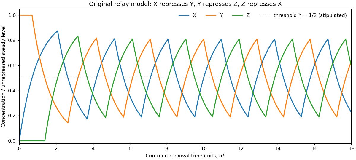
Original logic approximation for gene regulation trajectory of the repressilator, with threshold one half of the unrepressed level
. Details. Past exam of the biological physics course of the University of Oxford 2015 1 c Solution by Codex 0 2026-10-25
Codex 0 2026-10-25Normalize both fluorescent reporter intensities by their respective means, correcting unequal brightness and background, and denote them . Extrinsic gene-expression noise changes shared cellular conditions and moves both signals together: the scatter is a long narrow cloud around . Intrinsic gene-expression noise comes from distinct random expression events in the two genes and broadens the cloud across that diagonal. Comparable contributions therefore give a noticeably wider, still positively correlated cloud. The two right-hand panels in the preceding original illustration show these two cases.
For matched fluorescent reporters with conditionally independent intrinsic fluctuations and corrected measurement noise,The first quantity measures differential variation; the second measures common variation. A clone's successive observations can remain correlated in time, so they need not be independent samples. Shared activation transients should also be separated from the fluctuations of interest.[ref]
Stochastic Gene Expression in a Single Cell by Michael B. Elowitz and others. Science 297 (2002), pp. 1183–1186: dual-reporter discrimination of intrinsic and extrinsic variation
Past exam of the biological physics course of the University of Oxford 2015 1 b Solution by Codex 0 2026-10-25
Codex 0 2026-10-25With zero initial messenger RNA and protein concentration, solving the two linear ordinary differential equations in sequence givesThe last expression applies after the short messenger RNA transient when . All three mean curves have this shape. At a fixed steady state, a larger translational burst size requires fewer transcription events: . Thus gives infrequent large upward jumps followed by protein degradation, whereas gives many smaller jumps and a smoother trace.
Noise depends on molecule counts. If the fixed cell volume is , write . In the instantaneous-burst limit, independent Poisson process arrivals of geometrically distributed bursts, with count arrival rate , and unit protein degradation giveIndeed, the moment equations are and . With zero initial counts the variance becomes . These equations explain both the approach to the steady state and the scatter about it.
For illustration only, gives at the higher concentration: the two values of the coefficient of variation are and . At the lower concentration, and gives . Decreasing the concentration by a factor of 100 therefore increases relative fluctuations tenfold, despite keeping small bursts. Absolute fluctuation sizes cannot be inferred without a cell volume. The original sketches below stipulate that volume; they are model realizations, not source data.[ref]
Transient protein-count variance in the instantaneous-burst model. Derivation of the transient and stationary variance
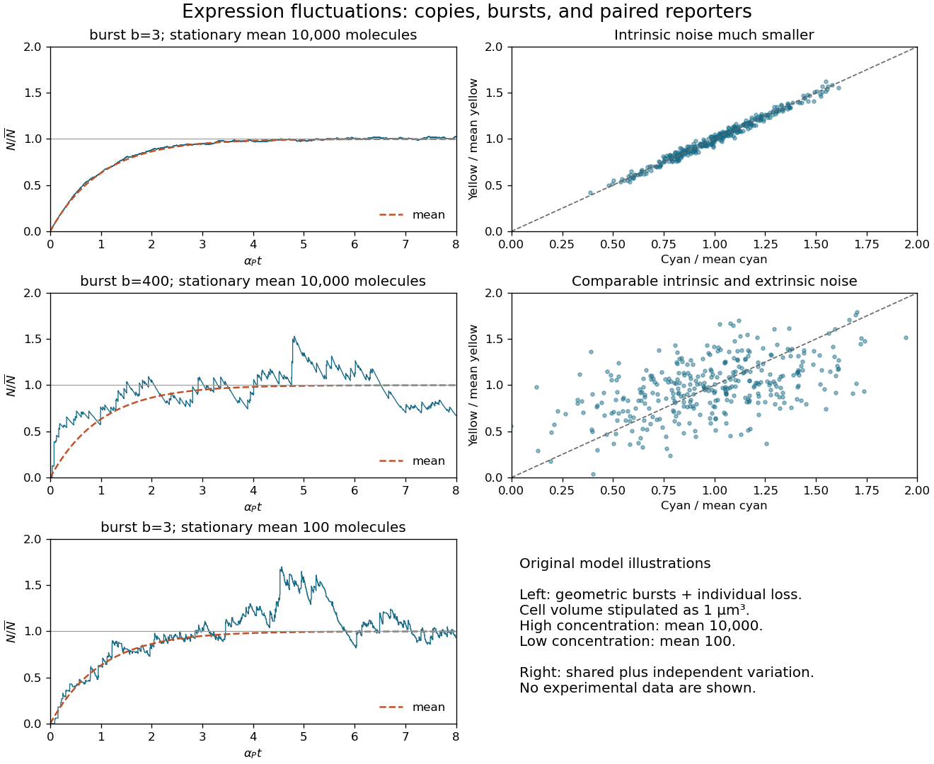
Translational burst size, relative expression fluctuations, and paired fluorescent reporters
. Details. Past exam of the biological physics course of the University of Oxford 2015 1 a Solution by Codex 0 2026-10-25
Codex 0 2026-10-25The messenger RNA has steady state . Since biological translation produces proteins at rate , setting the protein degradation rate equal to this production rate givesThe translational burst size is the expected number of proteins made during one messenger RNA lifetime, whose expected value is . It is dimensionless, rather than a production rate. With independent Poisson process translation and an exponential distribution for the lifetime, the resulting count has a geometric distribution on nonnegative integers with expected value and variance .
Past exam of the atomic and laser physics course of the University of Oxford 2022 4 d Solution by Codex 0 2026-10-25
Codex 0 2026-10-25For a closed absorbing two-level system, write , let , and use for the absorption cross section. This differs from the stimulated-emission cross section convention in part (a). With , the rate equations areAt steady state, for . Hence the positive absorption coefficient isFor the given sodium fine-structure transition, the statistical weights are , , so and . The small-signal transmission gives the optical depthTo account for the finite decrease of intensity through the sample, integrate rather than treating the stronger beam as exactly uniform. If , this givesTaking as the incident intensity and ,Using the photon energy then givesIgnoring the small variation of the stronger intensity would instead give about ; the integrated value uses the stated transmissions more consistently. The length is not needed to eliminate , but gives the check .
The resonant absorption cross section is of optical-wavelength-squared size, much larger than a typical atomic geometric collision area. Pressure broadening cross sections involve phase-changing interatomic encounters and need not equal hard-sphere collision areas; their numerical value depends on collision partners and speed. No precise ratio follows from the supplied data. A useful distinction is that resonant absorption involves coherent response on the optical scale, so its cross section need not resemble an chemical atom's geometric area.
For homogeneous spectral broadening, all participating chemical atoms must share the same resonance and single-atom response width. In a dilute sample dominated by natural linewidth, the weak-beam requirement isUsing the sodium atomic mass, equality occurs near , so is a sufficient thermal condition. Spatial Zeeman energy shifts, light shifts and transit effects should also be small, the laser should address the same selected component, and the interaction should last long enough for steady populations. Uniform impact pressure broadening can also be homogeneous, but would change the width and effective cross section; it is not included in the lifetime-only numerical model.
Real sodium also has hyperfine structure and optical pumping among magnetic sublevels. The inferred is the effective cross section of the stated two-level system model, assuming statistical sublevel populations and no loss into unaddressed states. A measurement on a resolved, polarized closed hyperfine structure component requires its actual transition dipole moment and selection rules; a universal polarization-independent sodium cross section cannot be inferred from this simplified model. The dependence of resonant cross sections and saturation intensities on sublevel preparation is tabulated explicitly for the real sodium D lines.[ref]
Sodium D Line Data by Daniel A. Steck. Section on saturation intensity and resonant scattering cross section, and Table 7
Past exam of the atomic and laser physics course of the University of Oxford 2022 4 c Solution by Codex 0 2026-10-25
Codex 0 2026-10-25Let and . Applying the integrated amplifier law to each section givesEliminating givesAs a consistency check, both amplifiers have . The second section receives a larger intensity and adds , compared with in the first, while its multiplicative optical gain is much smaller. This is the expected approach to constant extracted power in saturation.
Past exam of the atomic and laser physics course of the University of Oxford 2022 4 b Solution by Codex 0 2026-10-25
Codex 0 2026-10-25In a uniform steady amplifier, with no extra propagation losses, the local optical gain law givesIntegrate between the two faces of length to obtainFor , this reduces to exponential amplification. In deep saturation, the intensity increment approaches : finite pumping limits the extracted power.
Past exam of the atomic and laser physics course of the University of Oxford 2022 4 a Solution by Codex 0 2026-10-25
Codex 0 2026-10-25Define and let be the stimulated-emission cross section, averaged over upper magnetic sublevels. The Einstein coefficients relation gives the absorption cross section . Assume equally populated magnetic sublevels within each energy level, a steady pump, and a monochromatic beam. The photon flux is ; define and the effective population inversion . Then the rate equations areThe term includes both stimulated emission and absorption. In steady state, adding the two rate equations gives . The first equation then yieldsThe directed beam gains energy at rate per volume, giving and the optical gain coefficient . At line centre, write . ThereforeHere is the small-signal optical gain coefficient and is the saturation intensity, at which the local optical gain is half its small-signal value. Positive optical gain requires : the lower energy level must empty sufficiently quickly.
The cancellation of from is specific to this model's steady fixed pump and the fact that every upper spontaneous emission feeds the lower energy level. Adding an extra lower-state accumulation factor to would contradict these rate equations. Alternative conventions using the absorption cross section must replace by throughout. Homogeneous spectral broadening permits the whole selected ensemble to share this local saturation response.
Past exam of the atomic and laser physics course of the University of Oxford 2022 3 d Solution by Codex 0 2026-10-25
Codex 0 2026-10-25Use first-order time-dependent perturbation theory, setting in the equation for and retaining the generally complex matrix element . With and , the probability amplitude isFor , split the integral at the pulse maximum. For either or ,Thus the full first-order answer, without discarding the counter-rotating contribution, isAt long times it givesThis full expression is not exactly one squared Lorentzian line shape. To obtain the intended near-resonance spectral line profile, additionally assume , so the pulse has a narrow positive-frequency lobe and is negligible. ThenThe weak-excitation condition near resonance is . The squared Lorentzian line shape occurs because the symmetric exponential pulse has a Lorentzian line shape amplitude Fourier transform, which is then squared to obtain probability.
At half the maximum, , soThe full width at half maximum refers to varying the drive frequency through the positive-frequency resonance. For a concrete failure of the unqualified squared-Lorentzian line shape claim, set while keeping . The full first-order resonant probability is times the one-lobe prediction. Weak radiation alone therefore does not justify dropping the second Fourier transform lobe.
Past exam of the atomic and laser physics course of the University of Oxford 2022 3 c Solution by Codex 0 2026-10-25
Codex 0 2026-10-25Let the upper-state population lifetime be , and take the lower energy level to be stable. Spontaneous emission gives survival probability , hence a field or excited-state probability amplitude proportional to for . Its Fourier transform at angular frequency is proportional toThe squared modulus therefore has the Lorentzian line shapeHere is normalized over the full mathematical frequency axis. The full width at half maximum in ordinary frequency is . If both energy levels decay, their population decay rates add in the natural linewidth; pure dephasing adds to the amplitude-decay rate instead.
Impact-regime pressure broadening provides another example. Independent phase-randomizing collisions with rate give optical correlation proportional to , whose Fourier transform is a Lorentzian line shape of full width at half maximum . This assumes short, uncorrelated impacts: a general static distribution of perturbing fields need not give a Lorentzian line shape.
Past exam of the atomic and laser physics course of the University of Oxford 2022 3 b Solution by Codex 0 2026-10-25
Codex 0 2026-10-25Rabi oscillations require a coherent drive with a stable phase over several population cycles and an isolated, appreciably coupled pair of quantum states. For large-amplitude oscillations, the Rabi detuning must be comparable to or smaller than the Rabi angular frequency. The population lifetime, optical coherence time, transit time and drive coherence time should all exceed by enough to resolve the cycles. An ensemble also needs sufficiently uniform Rabi frequencies and Rabi detunings that phase averaging does not wash the oscillations out. The usual sinusoidal formula additionally assumes the rotating-wave approximation.
The Einstein coefficients describe incoherent transition rates, rather than the evolving optical probability amplitudes. Their simplest use is appropriate for broadband, randomly phased radiation, with field correlation time short relative to population evolution, or for rapidly dephased chemical atoms whose optical coherences can be eliminated. The radiation energy density per unit frequency must be smooth over the relevant spectral line. Stimulated upward and downward transitions and spontaneous emission then enter rate equations, without predicting coherent population return. A short observation time can give a small excitation probability even for a coherent field; that condition alone does not justify an Einstein coefficients rate description. Coherent laser irradiation can also admit steady rate equations after optical coherence has relaxed, with the appropriate saturation response.
Past exam of the atomic and laser physics course of the University of Oxford 2022 3 a Solution by Codex 0 2026-10-25
Codex 0 2026-10-25Choose the relative phases of the two energy eigenstates so that is real and nonnegative. Define the resonant Rabi angular frequency , the Rabi detuning , and . Substitution into the Schrödinger equation, followed by projection onto the two eigenstates, gives the exact interaction picture equationsKeep both probability amplitudes dynamical: replacing by one would incorrectly impose weak excitation and miss complete population transfer.
For , apply the rotating-wave approximation to discard the rapidly oscillating terms at . Differentiating the second remaining equation and using the first givesThe initial conditions are and . With , their solution isConsequently,This result permits order-one excitation, including full population transfer on resonance, even though the drive is small compared with the optical angular frequency.
For an average from switch-on to time , integrate the squared sine:On resonance this limiting average is , although the instantaneous probability repeatedly reaches one. The zero-coupling, zero-Rabi detuning case is understood separately as .
Near resonance alone does not make this an exact result for arbitrarily strong driving. The stated sinusoidal Hamiltonian also needs the rotating-wave approximation. A concrete counterexample is and : the exact equations give at switch-on, while the claimed rotating-wave sinusoid gives . Thus “without assuming weak radiation” can mean without assuming small excitation, but cannot remove the drive-to-carrier scale separation. The infinite-time average above belongs to the rotating-wave model; omitted corrections can accumulate over sufficiently long times.
Past exam of the atomic and laser physics course of the University of Oxford 2022 2 d Solution by Codex 0 2026-10-25
Codex 0 2026-10-25The remaining six positions give the other isotope's sequenceThe adjacent differences divided by are , respectively. Thus and the same endpoint argument gives .
For the same electronic energy level, the magnetic-dipole hyperfine structure constant is proportional to , to leading order in the small isotope-dependent change of the electronic wavefunction. Since the two nuclear spins are equal,Using the full spans averages over the approximate Landé interval rule: , soThe constants have the same sign, so the nuclear magnetic dipole moments have the same relative sign. Their absolute sign cannot be obtained from their ratio without the electronic field's sign. Finite nuclear-size corrections to the hyperfine interaction, often called the hyperfine anomaly, and electric-quadrupole corrections are neglected at this accuracy.
Past exam of the atomic and laser physics course of the University of Oxford 2022 2 c Solution by Codex 0 2026-10-25
Codex 0 2026-10-25Write , so the Landé interval rule for hyperfine structure intervals in ordinary frequency is . For the first four selected positions, the successive positive differences areTheir ratios are approximately , sinceThe decreasing frequencies therefore correspond to increasing , with , if increasing printed position means increasing physical frequency. Continuing the intervals predicts additional positions near and then . They identify peaks and unambiguously. The full assignment for isWith , these endpoints requireEquivalently, a complete set of six hyperfine levels gives when . This inference assumes that every upper hyperfine level contributes an observed position and the negligible lower hyperfine structure lets coincident transitions be grouped by their upper energy. A line count without these completeness assumptions would not alone fix nuclear spin.
The supplied positions obey the Landé interval rule only approximately. For example, , whereas . Even allowing each printed position a rounding error of does not fully reconcile these two relations. A least-squares dipole-only fit has a largest position residual of about . Small additional hyperfine interactions, measurement uncertainty beyond the displayed precision, or an error in the tabulated data could account for this; it is inappropriate to claim an exact identity. The grouping and nuclear spin are nevertheless robust. Reversing the convention for the printed frequency axis reverses the inferred signs of both constants, without changing the following ratio.
Past exam of the atomic and laser physics course of the University of Oxford 2022 2 b Solution by Codex 0 2026-10-25
Codex 0 2026-10-25The shell carries a large spin (its ground atomic term under Hund's rules has ), and the electron penetrates the inner shells. Its nonzero probability density at the atomic nucleus supplies a potentially large Fermi contact interaction with the nuclear magnetic dipole moment. The shell here is singly occupied, so the obligatory paired- cancellation is absent. Both stable europium isotopes have nonzero nuclear spin, as the spectrum below also establishes.
The term symbol specifies , , . Its large , combined with appreciable nuclear spin, permits a wide range of total angular momentum and hence a substantial total hyperfine structure span. For , and the span is . The penetrating contribution and the available range of explain the large hyperfine structure; the term symbol alone does not determine its constant, which also depends on electronic recoupling, radial wavefunctions and configuration interaction.
Past exam of the atomic and laser physics course of the University of Oxford 2022 2 a Solution by Codex 0 2026-10-25
Codex 0 2026-10-25Let the dimensionful angular momentum operators obey and take the interaction Hamiltonian as . Sincethe energy eigenvalues at fixed arewhere . Subtraction gives the Landé interval ruleMany atomic conventions use dimensionless angular momentum operators and call the energy-valued constant itself ; then the right-hand side is . Each energy level has magnetic sublevels with the same energy in zero field.
For fine structure, the effective interaction is with dimensionless angular momentum operators. It originates in the spin-orbit interaction, including the magnetic interaction of electron spin with orbital motion and its relativistic correction. Within an isolated LS coupling atomic term, the labels are the electron configuration, , and the interval between adjacent energy levels is . This is smaller than the electrostatic separation of atomic terms.
For magnetic-dipole hyperfine structure, the nuclear magnetic dipole moment interacts with the magnetic field generated by the electrons. Contributions include the Fermi contact interaction of penetrating electrons, orbital magnetic fields, and the dipolar field of electron spin. Projected onto one electronic energy level, their rotationally invariant magnetic-dipole part has the form . The labels are , together with the approximate electronic labels such as . This splitting is generally smaller than fine structure, reflecting the much smaller nuclear magnetic dipole moment. An electric nuclear quadrupole moment can add a different interaction and violate the simple Landé interval rule.
At the larger electrostatic energy scale, an effective two-spin exchange interaction can also be written within fixed orbitals. Its origin is the Coulomb interaction combined with the Pauli exclusion principle, rather than a large direct magnetic interaction. It separates singlet state and triplet state atomic terms; before spin-orbit coupling, useful labels include the electron configuration, . General electrostatic atomic term separations need not obey a single Landé interval rule as varies.
Past exam of the atomic and laser physics course of the University of Oxford 2022 1 d Solution by Codex 0 2026-10-25
Codex 0 2026-10-25The closest components above differ by . At , their separation is about . A visible spectral line near would consequently require spectral resolving power of order . An ordinary low-resolution spectrometer would merge the components.
A suitable arrangement places an excited low-pressure strontium discharge or a transversely observed atomic beam between wide electromagnet pole pieces. Collect the emission perpendicular to the magnetic field, select the desired spectral line with a prefilter or monochromator, and send it through a high-finesse scanning Fabry–Pérot interferometer to a detector. A rotatable linear polarizer separates the two components from the four components. Calibrate both the interferometer's free spectral range and the local magnetic field; take zero-field and several field-strength scans, and fit component positions against .
The magnetic field should be uniform across the viewed volume, with its associated Zeeman splitting larger than the combined natural linewidth, Doppler broadening, pressure broadening and instrumental width, but much smaller than the separations of the relevant atomic fine-structure levels. A collimated transverse atomic beam, low collision rate and restricted collection angle reduce unwanted spectral line broadening. Avoid appreciable power broadening, resolve or model isotope and hyperfine structure, and check for self-absorption. A zero-field scan and the predicted linear scaling help distinguish actual Zeeman splitting components from neighbouring spectral lines.
Pinned article: Introduction to the OurBigBook Project
Welcome to the OurBigBook Project! Our goal is to create the perfect publishing platform for STEM subjects, and get university-level students to write the best free STEM tutorials ever.
Everyone is welcome to create an account and play with the site: ourbigbook.com/go/register. We belive that students themselves can write amazing tutorials, but teachers are welcome too. You can write about anything you want, it doesn't have to be STEM or even educational. Silly test content is very welcome and you won't be penalized in any way. Just keep it legal!
Intro to OurBigBook
. Source. We have two killer features:
- topics: topics group articles by different users with the same title, e.g. here is the topic for the "Fundamental Theorem of Calculus" ourbigbook.com/go/topic/fundamental-theorem-of-calculusArticles of different users are sorted by upvote within each article page. This feature is a bit like:
- a Wikipedia where each user can have their own version of each article
- a Q&A website like Stack Overflow, where multiple people can give their views on a given topic, and the best ones are sorted by upvote. Except you don't need to wait for someone to ask first, and any topic goes, no matter how narrow or broad
This feature makes it possible for readers to find better explanations of any topic created by other writers. And it allows writers to create an explanation in a place that readers might actually find it.
Figure 1. Screenshot of the "Derivative" topic page. View it live at: ourbigbook.com/go/topic/derivativeVideo 2. OurBigBook Web topics demo. Source. - local editing: you can store all your personal knowledge base content locally in a plaintext markup format that can be edited locally and published either:This way you can be sure that even if OurBigBook.com were to go down one day (which we have no plans to do as it is quite cheap to host!), your content will still be perfectly readable as a static site.
- to OurBigBook.com to get awesome multi-user features like topics and likes
- as HTML files to a static website, which you can host yourself for free on many external providers like GitHub Pages, and remain in full control

Figure 2. You can publish local OurBigBook lightweight markup files to either OurBigBook.com or as a static website.
Figure 3. Visual Studio Code extension installation.
Figure 5. . You can also edit articles on the Web editor without installing anything locally. Video 3. Edit locally and publish demo. Source. This shows editing OurBigBook Markup and publishing it using the Visual Studio Code extension. 
- Infinitely deep tables of contents:




All our software is open source and hosted at: github.com/ourbigbook/ourbigbook
Further documentation can be found at: docs.ourbigbook.com
Feel free to reach our to us for any help or suggestions: docs.ourbigbook.com/#contact