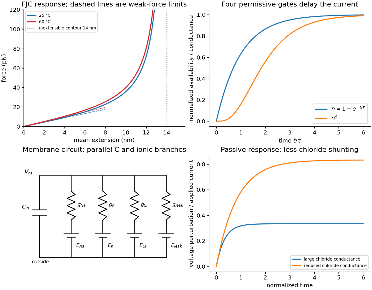
This is an increase by about 11.7%. The factor kBT multiplies the free energy penalty for the loss of chain configurations; a larger force is required to impose the same normalized weak extension at higher temperature.
Not degrading does not guarantee that a real protein's folded state, effective spring constant or solvent interactions remain unchanged. Thermal unfolding and changes in persistence length can occur without covalent degradation. Those changes modify the experimental curve and may invalidate a fixed-N,b comparison. The boxed value is the explicit ideal-FJCprediction under fixed segment geometry, not an unconditional thermal-stabilityprediction for the protein.
At moderate force, even an ideal FJC becomes nonlinear as its orientations align, so failure of a linear fit alone need not imply nonideal chemistry. But failure of the full FJCcurve can reflect backbone spring constant and correlated segment angles, nonuniform effective links, remaining folded contacts, force-induced conformational changes, energetic bond compliance, or tether/calibration effects. An extensible FJC or an appropriate semiflexible model includes some of these effects; their parameters require independent justification. The stated inextensible 14nmpolymer contour length already excludes a literal 15nm extension.
The first panel of the original model figure below shows the full orientational response and weak-forcetangents without tracing the experimental data.
The controlled weak-force condition is fb≪kBT, not merely that a short part of a measured curve looks straight. With the supplied b, kBT/b≃10.3pN at 25∘C. A raw force near 30pN, as in the figure's labelled low-extension portion, would give u≃2.9 and is not asymptotically weak for those literal segment parameters. A force offset or different effective model might change that interpretation, but no such correction should be invented from the plot.
The AFM pulls a tethered molecule through its cantilever. Deflection, multiplied by a calibrated cantileverspring constant, measures force; supportmotion must be corrected for that deflection and any linker compliance to obtain molecular extension. Initially folded structure can resist extension, then contacts break and more polypeptidepolymer contour length becomes available. The readable trace rises with increasing extension, with fluctuations and a strongly rising large-extension part. It should not be interpreted asa direct image of individual amino acids or as establishing a unique microscopic unfolding pathway.
Its mean extension is strictly below 14nm at every finite force. Thus the quoted 15nm maximum does not establish ideal FJC behaviour: if both numbers are taken literally, it exceeds the model's polymer contour length by about 7%. Finite segment stretch, inaccurate effective segment parameters, additional linkers or an extension-zero/calibration error can account for such adifference. If the numerical descriptions are approximate, the discrepancy may be within their uncertainty; even exact agreement with a polymer contour length would not prove freely jointed statistics. Low-force fluctuations and the full force–extension relation are separate tests.
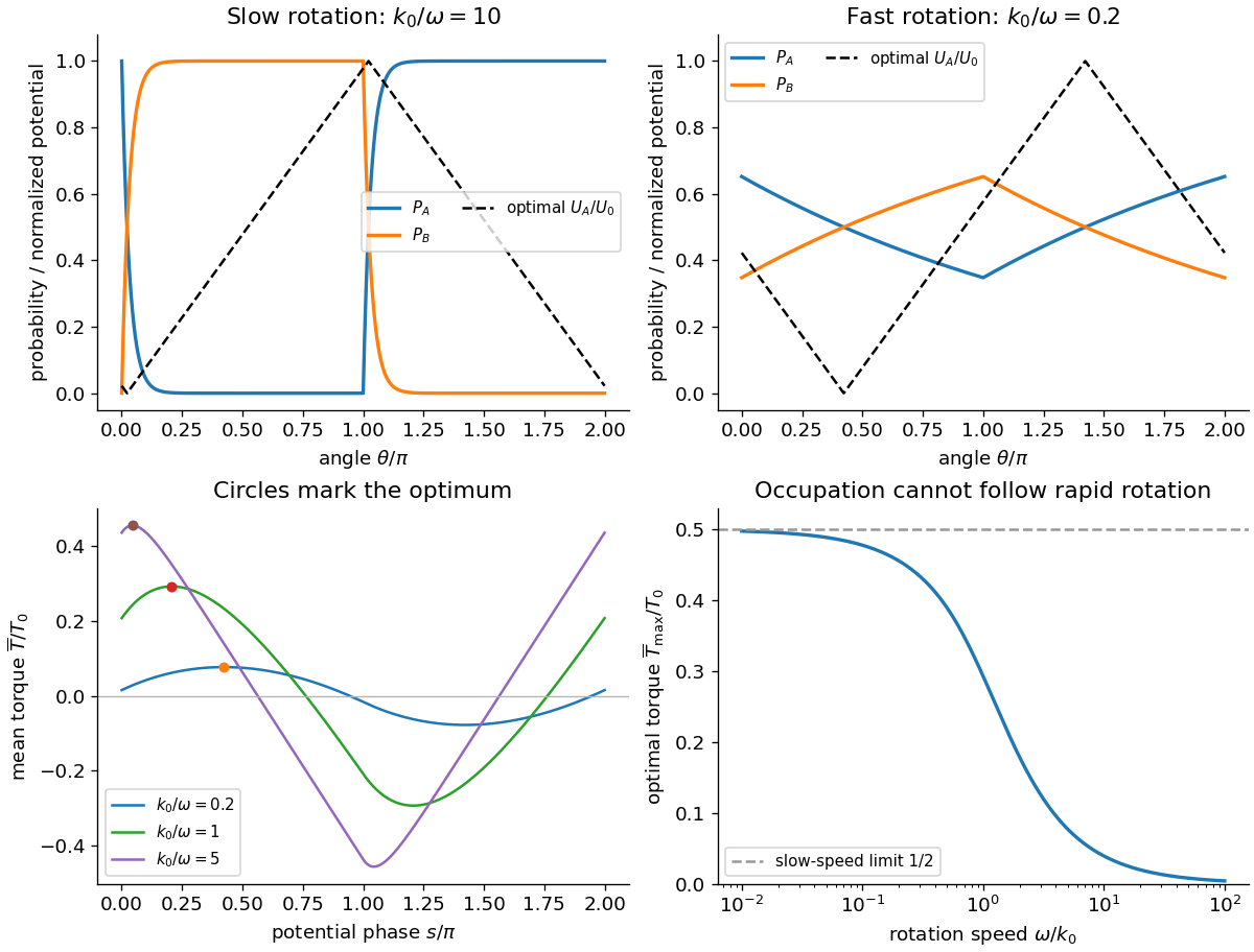
The source potential rises from zero to U0 over the half-turn from s to s+π, then falls over the next half-turn. Its slopes are ±U0/π. Torque is minus the angular derivative of potential; in the detached state UB is angle-independent and exerts no torque. A uniform set of motor phases therefore gives
The crossing displaced by π is the corresponding minimum. For slow positive rotation, smax≃(ω/k0)ln2 lies just after the detachment switch. The potential then rises mainly while the motor is detached and falls mainly while it is bound. For fast rotation, smax≃π/2−π2k0/(8ω), with only a small phase-dependent occupation available to produce torque. The potential should still be shifted by this optimum, rather than aligned arbitrarily with a rate switch.
The half-turnsymmetry gives ∫ss+2πPAdθ=π. At the optimum, direct integration of the two exponential pieces gives ∫ss+πPAdθ=smax. Thus auseful exact check is
For fast rotation, Tmax≃T0πk0/(8ω) instead tends to zero. The original plots below show the calculated probabilities and optimized potential shapes. The imposed switching rates constitute driven kinetics: their strictly one-way windows are not equilibriumdetailed balance at a fixed angle. Sustained work requires the motor's chemical/ion-gradient energy supply, not extraction of work from a passive single thermal bath.
Motor occupation, optimal angular potential phase and the speed dependence of available torque
. Original solutions of the two-state advective motor model. Potential is normalized by U0, torque by T0, and the slow/fast profiles use illustrative values of k0/ω. Details.
In particular PA(0)=PA(2π)=α and PA(π)=1−α, so the two pieces fill in the apparent endpoint gap in the printed piecewiseformula. The probability decreases exponentially during the detachment half-cycle and rises exponentially during the attachment half-cycle; PB is its complement. Both remain between zero and one. They are state probabilitiesconditional on rotor angle, not separate angular densities normalized individually to one.
For ω≪k0, attachment and detachment almost finish within their allotted half-turns: PA is nearly zero through most of 0<θ<π and nearly one through most of π<θ<2π, with angular boundary layers of width ω/k0. For ω≫k0, it stays near one half with a small nearly triangular modulation. The upper panels of the original figure in part (b) sketch both limits. At exactly zero speed the advective stationary problem is singular; these statements concern the positive-speed limit.
Coupling is essential: an overall favourable reaction can drive an unfavourable one only when their processes are linked, rather than merely present in the same cell. At fixed conditions the extracted work is bounded by the consumed free-energy decrease. Dissipation produces heat and entropy, so energy conservation does not mean all energy remains available for work. Thermal fluctuations can drive random motion, but a persistent directional cycle requires a nonequilibrium free-energy source; an equilibrium asymmetric structure alone is not afree motor.
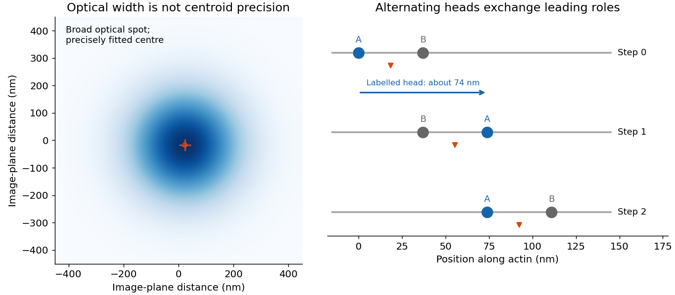
In myosin-V tracking, localizing a label on one head or its lever arm distinguishes the paths of individual motor parts from the averagemotion of the whole motor. A trailing head that becomes the leading head travels roughly twice the stalk advance: about 74nm versus a roughly 37nm motor stride. A near-head label can therefore alternate a large movement with a pause while the partner head advances. Other lever-arm label positions give unequal alternating steps whose sum is approximately twice the stride. Those patternssupport hand-over-hand walking rather than a simple inchworm model in which the same head remains in front. The label geometry is needed when interpreting individual step sizes.[ref]
A fitted diffraction spot can locate alternating myosin heads beyond its optical width
. An original Gaussian spot illustrates the distinction between point-spread width and centre precision. A separate schematic shows a labelled head alternating a roughly 74-nanometre movement and a pause while the two-head motor advances in roughly 37-nanometre strides. It is a conceptual calculation, not copied tracking data. Details.
Super-resolutionlocalization microscopy extends the same principle to amap containing many molecules by separating otherwise overlapping emitters in time. Sparse activation, blinking or transient binding yields individually fitted positions, which are accumulated. Dense sampling, registration and labelling specificity determine the final structural resolution; merely taking more photons from an unresolved simultaneous pair does not make it a single isolated emitter.
In PAINT, fluorescent probes bind transiently so that separated binding events can be localized and accumulated. DNA-PAINTuses reversible complementary-strand recognition at docking sites on a DNAnanostructure. The bound probe supplies a localized spot while freely diffusing probes contribute background; repeated visits build up a positional map, with replenishment rather than permanent reliance on one fluorophore. This is an imaging principle, not a requirement for a particular target sequence or preparation protocol.[ref]
Independent localization errors of varianceσloc2 add an intercept 2σloc2. Finite exposure adds motion blur, and drift, binding transitions and the finite DNA contour must be distinguished from free sliding. Aslope fit with those limitations can estimate D1; simply fitting all observed displacements to a noiseless line can bias it.
Consequently no fluorescencecamera could temporally resolve trajectories under the stated formal values, regardless of the spatial excursion'slength. An actual corrected exponent cannot be inferred uniquely from the paper. If a physically plausible D1 were supplied instead, resolving sliding would require exposures substantially shorter than τbound and diffusiondisplacements larger than localization error, with enough detected photons. The dependence on D1 is explicit above, so no guessed source correction is needed.
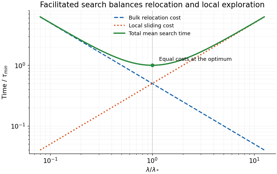
Write A=V/D3 and B=L/D1. The given mean-search scaling is τ=A/λ+Bλ. Three-dimensional relocation sees an effective capture length of order λ, givinga bulk encounter time V/(D3λ). A sliding excursion explores length of order λ in time of order λ2/D1; sampling order L/λ contour segments gives a total sliding cost of order Lλ/D1. Prefactors, correlations and repeated visits are coarse-grained in this scaling model.
Small slidinglengths make relocation inefficient; very long slidingwastestime revisiting a local DNA region rather than relocating to another. The optimum balances both contributions:
Bulk relocation and local sliding impose opposing search-time costs
. The original dimensionless plot shows a decreasing inverse-sliding-length contribution and an increasing sliding contribution. Their sumhas a minimum where the two costs agree, at a sliding length equal to the analytic optimum. Details.
The model is meaningful only over an accessible range between molecular steps and the available chromosomelength. An optimum outside that range is replaced by a boundary choice; the unphysical divergences at arbitrarily small or large λ describe limits of the scaling expression. A common multiplicative searcher-number factor would not change the optimum, but an exact many-searcher first-arrival mean is not generally obtained by dividing an arbitrary single-searcher mean by their number without a waiting-time assumption.
Model the target asa perfectly absorbing sphere of reaction radius r0, with a fixed target and a dilute far-field polymerase density c∞. Steady radial diffusion satisfies ∇2c=0, c(r0)=0, c(∞)=c∞, hence
This is an idealized 10−2-second-scale estimate, not a unique geometric prediction. Finite cellshape, crowded motion, accessibility and orientational restrictions can reduce the ideal capture rate.
If nonspecific binding merely sequesters searchers and their freefraction is 0.2, the three-dimensional capture hazard is reduced fivefold: τ≃τ3/0.2≃0.067s for those estimates. If bound molecules instead search productively by sliding, afree-timefraction alone cannot determine the total arrival time or its sign of change. That is the distinct facilitated-search mechanism treated in c.
At initiation, RNA polymerase recognizes a promoter and forms a closed bound complex; bacterial promoter recognition involves its specificity factor. Local strand opening exposes the template in an open complex, after which initial RNA synthesis can precede promoter escape into elongation. Binding, opening and productive escape are distinct transitions.
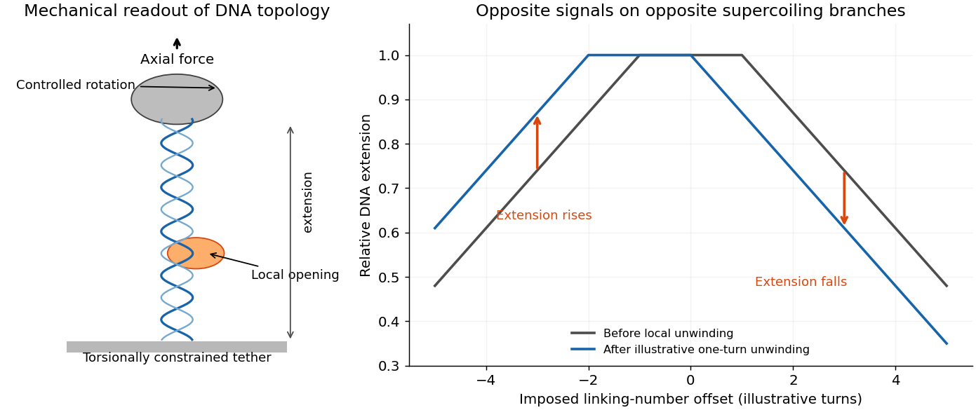
Opening a small helical region decreases twist, so the rest of the tether acquires compensating positive writhe. On a negatively supercoiledtether this removes some writhe magnitude and raises its extension; on a positively supercoiledtether it increases writhe magnitude and lowers extension. A change with opposite signs under the two torsional conditions therefore distinguishes unwinding from simple compaction, which would shorten both tethers. Calibrating extension against imposed turns converts a mechanical step into a change in helical winding. This is a conceptual readout of local opening, rather than a direct optical image of separated bases.[ref]
Torsional constraint converts local DNA opening into a bead-extension signal
. An original conceptual magnetic-tweezers schematic is paired with illustrative extension-versus-turns curves. Local unwinding shifts the curve and produces opposite extension changes on its negatively and positively supercoiled branches. The diagram does not reproduce the source experiment or specify alaboratory protocol. Details.
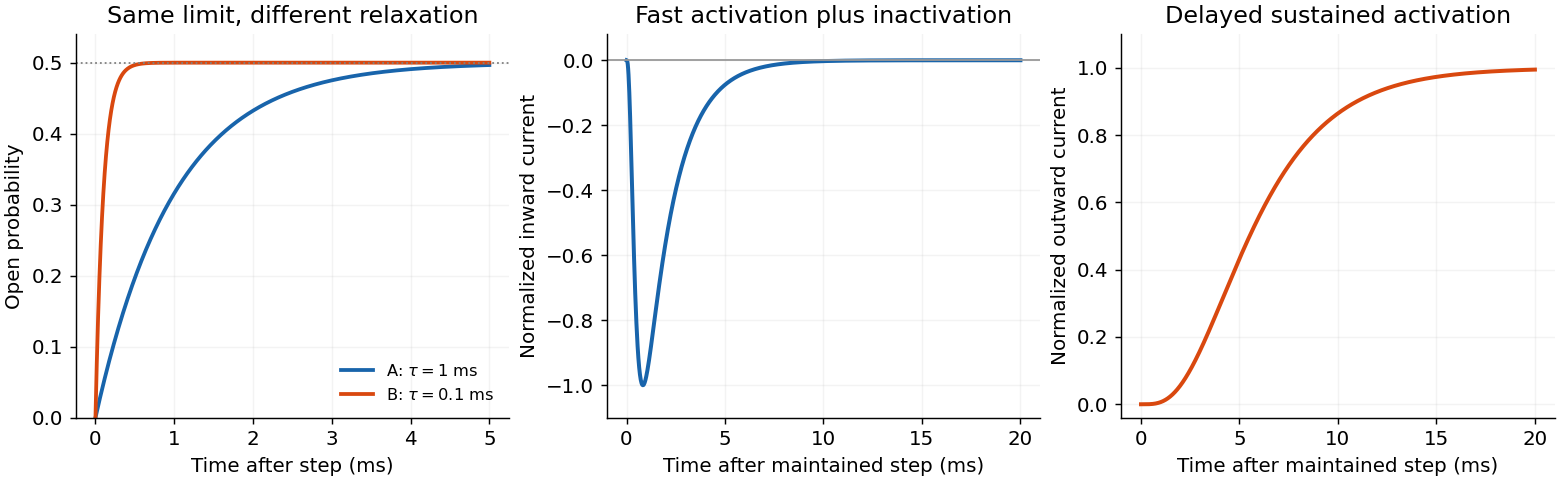
A two-state closed–open scheme at fixed voltage relaxes monotonically and cannot by itself produce asodium-current transient during a maintained step with constant driving force. A minimal sodiumscheme therefore includes an unavailable state: C⇄O⇄I, with voltage-dependent activation, inactivation and recovery; closed-state recovery pathways may be added when needed. Opening is initially rapid, occupancy then accumulates in I, and recovery on repolarization restores an activatable population.
For the illustrated potassium current, a closed–open model gives sustained opening, but several activation steps can account for its initial delay. A conventional illustrative coarse-grained description is
with each gate following q˙=αq(V)(1−q)−βq(V)q. Fast mactivation, subsequent decrease of h, and slower increase of n produce the two qualitative records. The powers are phenomenological gate assumptions, not values uniquely inferred from these traces or an exact structural count for every cardiac channel.
A1-Hz cardiac rhythm has about asecond between successive activations, whereas a100-Hz neuronal rhythm has only 10ms; the available resting interval is shorter still after subtracting the action potential. Recovery or deactivation with a timescale comparable to that interval can then leave residual inactivation or potassiumactivation, giving use-dependent changes and refractoriness. Millisecond or faster relaxation usually completes much more readily during a long diastolic interval. The particular two-stateA and B in d would both nearly equilibrate over a full 10ms at their stipulated constant rates; their values alone do not demonstrate high-frequency failure. Real comparison requires voltage-dependent recovery rates and the different cardiac and neuronal waveforms. A frozen-rate model cannot quantitatively predict either firing pattern from frequency alone.
An individual channel remains either open or closed. Its mean closed and open dwell times are 1/a and 1/b, respectively: both are 2ms in A and 0.2ms in B. Thus identical equilibrium open probability does not imply identical kinetics or noise correlationtime. Ensemble probability relaxation depends on the sum of rates, while the mean dwell in a given state depends on its exit rate.
An increased late inward sodium current can delay repolarization if fast inactivation is incomplete or slowed, if channels reopen excessively, or if the voltage range of persistent/window current is enlarged. A larger brief peak current alone is not equivalent to a sustained depolarizing current. Conversely, reduced outward potassium current can prolong the action potential through fewer functionalsurfacechannels, reduced conductance, slower or less favourable activation, or altered deactivation/availability. Either change shifts the balance towards inward current during repolarization.
These are distinct biophysical routes to Long QT syndrome, not claims that every subtype has the same channel defect.[ref]
A sodium-channel alpha subunit contains four homologous domains assembled into one pore, with separate voltage sensors. Rapid activation and fast inactivation are distinguishable conformational transitions; an intracellular inactivation apparatus stabilizes nonconducting states after activation. Repolarization favours recovery of availability. A channel can therefore be closed but activatable, or inactivated and temporarily unavailable, despite zero current in both cases.
These observations constrain models but do not make an individual macroscopic trace a unique structural reconstruction. Different distributions of closed and inactivated states can produce similar averages. In particular, the sustained potassium trace supports little inactivation on the displayed interval; it does not justify assigning every potassium channela universal absence of an inactivation mechanism.
After a domain unfolds, its backbone joins the same continuous chain as previously unfolded material. The new branch differs mainly by an added contour length, while the local backbone bendingstatistics remain similar. It is therefore consistent to fit successive branches with different Lj and one common Lp≃0.8nm. Tension is transmitted through serial portions of the same chain; one should not add their tensile forcesas though they were independent parallel springs.
The persistence length is short compared with the contour increment per repeat, so each released domain contributes many flexible bending segments. Stretching suppresses those thermal modes and raises free energy through loss of entropy, which is precisely the worm-like-chain mechanism. The common Lp is a property of the unfolded backbone under the measurement conditions, not the folded domain's axial length or the number of domains already released. With T=300K only as an illustrative value, kBTLp≃3.3pNnm2.
A common persistence-length fit is evidence for approximately repeat-independent chain flexibility over the observed branches; it is not proof that a continuum inextensible model describes every molecular scale. Residual folded structure, heterogeneous linkers, force-induced backbone stretching, and very short-chain effects can cause deviations. The formal forcedivergence at x=Lsignals the model's inextensibility assumption, not a physical infinite tensile force.
For small extension, expansion gives f≃[3kBT/(2LpL)]x, so the effective entropic spring constant is 3kBT/(2LpL). Close to full extension, f∼kBT/[4Lp(1−x/L)2], giving strong strain stiffening. These regimes constrain the fit differently and correlate its parameters if the measured interval is short. The fit does not by itself identify a unique folding barrier or unfolding kinetic rate.
Welcome to the OurBigBook Project! Our goal is to create the perfect publishing platform for STEM subjects, and get university-level students to write the best free STEM tutorials ever.
Everyone is welcome to create an account and play with the site: ourbigbook.com/go/register. We belive that students themselves can write amazing tutorials, but teachers are welcome too. You can write about anything you want, it doesn't have to be STEM or even educational. Silly test content is very welcome and you won't be penalized in any way. Just keep it legal!
a Q&A website like Stack Overflow, where multiple people can give their views on a given topic, and the best ones are sorted by upvote. Except you don't need to wait for someone to ask first, and any topic goes, no matter how narrow or broad
This feature makes it possible for readers to find better explanations of any topic created by other writers. And it allows writers to create an explanation in a place that readers might actually find it.
This way you can be sure that even if OurBigBook.com were to go down one day (which we have no plans to do as it is quite cheap to host!), your content will still be perfectly readable asa static site.
 Codex 0 2026-10-25