The gradient and quadratic terms of the stated model balance at the amplitude-variation scale $\xi$. It is a superconducting length scale, distinct from optical coherence length. The weak-field London penetration depth in the same normalization obeysA core suppresses the pairing amplitude over a scale set by $\xi$; screening electric currents and the magnetic field involve $\lambda$. Neither scale is a universal particle size.

A concrete motivating experiment is the acetone–chloroform mixture in Truman State University's Liquid-Vapor Equilibrium of a Binary System, Procedure and Figure 1. A two-neck flask feeds a distillation head with a water-cooled laboratory condenser, condensate sampling arm and temperature probe. Starting with one pure liquid, the procedure adds the other component successively and waits for stable temperature with returning condensate. Small paired samples from the flask and condensate are read on an Abbé refractometer; a tabulated refractive index–composition relation gives the two compositions. Controls include three-point thermometer calibration, corrected atmospheric pressure readings, and agreement of the initial pure-liquid and condensate refractive indices with the reference value. Small withdrawals and little retained condensate reduce disturbance of composition. Sample evaporation can bias the readout. The inferred paired mole fractions, temperature and pressure describe vapor-liquid equilibrium, subject to the conversion from mass fraction to mole fraction and to representative sampling. This teaching protocol reports no measured results of a particular student run.^[ref]

How does such a measurement expose activity coefficients? Let $x_i$ and $y_i$ be the mole fractions in the liquid and gas thermodynamic phases, respectively, and let $p_i^{\ast }(T)$ be the pure-component vapor pressure. Assume the gas thermodynamic phase is an ideal gas mixture and neglect the change of the pure-liquid reference chemical potential between its saturation pressure and the experimental pressure. Equality of each component's chemical potential between the two thermodynamic phases then givesThis turns the paired composition readings into estimates of the activity coefficients. The approximation needs refinement when the gas departs appreciably from ideal gas behavior or the neglected liquid pressure effect matters.

The apparatus measures a boiling-composition series in which temperature changes as the mixture changes. Its readings therefore cannot be inserted directly into the fixed-temperature, fixed-pressure activity coefficient constraint. They motivate the more general task: test whether the measured mixture properties can arise from a common Gibbs free energy while accounting for changing state variables. A failure can reveal incompatible property fits or experimental bias; a pass supplies a consistency check, not proof that every reading is correct.

For a nonideal chemical solution, write its thermodynamic activities on a mole fraction basis as $a_A=x{\gamma }_A$ and $a_B=(1-x){\gamma }_B$. Use composition-independent pure-component reference chemical potentials at the same temperature and pressure:The activity coefficients describe departure from the ideal solution under that reference convention.^[ref]

At fixed temperature and pressure, insert these expressions into the Gibbs-Duhem equation. The ideal solution terms cancel because $xd\ln x+(1-x)d\ln (1-x)=dx-dx=0$. What remains isThus two independent fits to measured activity coefficients can each look smooth while failing to describe one possible Gibbs free energy. This is a necessary consistency condition; satisfying it alone does not establish experimental accuracy or thermodynamic stability.

For an original algebraic example, suppose at one fixed temperature and pressure that $\ln {\gamma }_A=\alpha (1-x{)}^2$, with dimensionless constant $\alpha$. The constraint requires $d\ln {\gamma }_B/dx=2\alpha x$. With the pure-B normalization ${\gamma }_B(0)=1$, integration givesFor $\alpha =1/2$ and $x=1/4$, the derivatives of the two logarithms are $-3/4$ and $1/4$; their weighted sum is $-3/16+3/16=0$. Choosing $\ln {\gamma }_B=\alpha x$ instead would give a weighted sum $3/16$ at that composition, contradicting the Gibbs-Duhem equation. These are invented model functions, with no claim to fit a particular mixture.

The fixed-temperature, fixed-pressure restriction matters. Along a path with changing temperature or pressure, the general equation contains $SdT-Vdp$, and the reference chemical potentials and $RT$ also change. Across phase coexistence, apply the relation separately within each smooth thermodynamic phase; do not differentiate a discontinuous switch between phases as if it were a single composition curve.

An ideal solution has molar chemical potentialswhere $R$ is the molar gas constant and the stars denote pure-component reference values at the same temperature and pressure.^[ref]

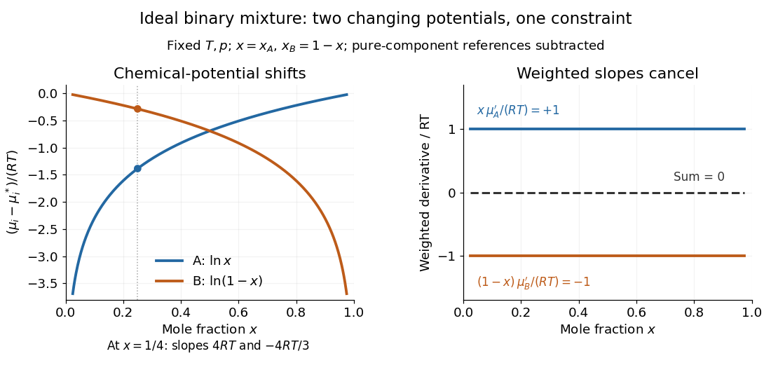
Hold temperature and pressure fixed. The derivatives with respect to $x$ are $RT/x$ and $-RT/(1-x)$, soEach chemical potential changes, yet their composition-weighted slopes cancel exactly. At $x=1/4$, the two slopes are $4RT$ and $-4RT/3$; multiplying by $1/4$ and $3/4$ gives $RT$ and $-RT$. Near either pure-component endpoint the dilute component's slope diverges, but its weighted contribution remains finite. The endpoint chemical potential itself requires a limiting interpretation because its logarithm diverges.

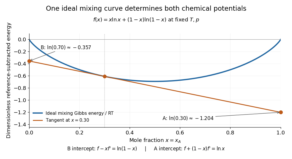
The same constraint has a geometric explanation. Subtract the pure-component reference contribution from the molar Gibbs free energy and divide by $RT$ to obtainIts derivative is $f^{\prime }(x)=\ln [x/(1-x)]$. At fixed total amount of substance, exchanging a little B for A changes the Gibbs free energy with slope ${\mu }_A-{\mu }_B$. Consequently the tangent to $f$ at $x$ has interceptsat horizontal coordinates $0$ and $1$, respectively. The two chemical potentials come from the same curve: choosing two unrelated functions would generally destroy this tangent construction.

The real invertible matrices with positive determinant form a subgroup of the general linear group. The identity has determinant one, multiplicativity of the determinant preserves positivity under products, and $\det (A^{-1})=1/\det A>0$ preserves it under inversion. More precisely this is the kernel of a group homomorphism $A\mapsto \mathrm{sgn}(\det A)$ to $\{1,-1\}$, so it is a normal subgroup of index two for $n\ge 1$. Its elements preserve an orientation of a vector space.

Let the initial Gaussian wave packet beFourier transforming, multiplying each momentum amplitude by $e^{-i{p}^{2}t/(2m\hslash )}$ and evaluating the Gaussian integral givesIts probability density is a normalized Gaussian with center $x_0+p_{0}t/m$ and width ${\sigma }_x={\sigma }_0\sqrt{1+{\eta }^2}$; the momentum width remains ${\sigma }_p=\hslash /(2{\sigma }_0)$. Its symmetrized position-momentum covariance is $C_{xp}=t{\sigma }_p^2/m$, soThus free spreading preserves equality in the Robertson-Schrödinger uncertainty relation while producing a nonzero quadratic position-dependent phase and a product ${\sigma }_x{\sigma }_p$ larger than $\hslash /2$. More generally, ${\sigma }_x(t{)}^2={\sigma }_x(0{)}^2+2t{C}_{xp}(0)/m+t^2{\sigma }_p(0{)}^2/m^2$, so an initially correlated Gaussian can first contract.

Under a quantum harmonic oscillator Hamiltonian, the Heisenberg equations of motion giveSubtract the expectation values, square the first equation, and use the symmetrized covariance $C_0=⟨\{x-⟨x⟩,p-⟨p⟩\}⟩/2$. This yieldsThese moment equations hold for any state with finite second moments; a quadratic Hamiltonian additionally preserves Gaussian wave packets. A coherent state has ${\sigma }_x(0{)}^2=\hslash /(2m\omega )$, ${\sigma }_p(0{)}^2=m\hslash \omega /2$, and $C_0=0$, so its width stays fixed while its center follows the classical orbit. A squeezed coherent state generally has a width that oscillates at $2\omega$.

For $H=-d^2/d{x}^2+x^2+ϵx^4$, use the normalized real wavefunction ${\psi }_{\alpha }=(\alpha /\pi {)}^{1/4}{e}^{-\alpha x^2/2}$, $\alpha >0$. The Gaussian integral gives $⟨x^2⟩=1/(2\alpha )$ and $⟨x^4⟩=3/(4{\alpha }^2)$, while the kinetic contribution is $\alpha /2$. Thus the Rayleigh quotient is the displayed expression. For positive $ϵ$, its stationary width satisfies ${\alpha }^3-\alpha -3ϵ=0$. At $ϵ=2$ the unique positive solution is $\alpha =2$, giving $E_0\le 13/8$ by the Rayleigh-Ritz variational principle. For $ϵ<0$, taking $\alpha \downarrow 0$ makes the negative quartic contribution dominate, so the energy is unbounded below even within this normalized family. The positive-coupling bound and negative-coupling instability concern different signs of the same variational expression.

For a smooth axisymmetric magnetic field, write $B_z(\rho ,z)=B_0(z)+O({\rho }^2)$. The absence of magnetic monopoles gives ${\rho }^{-1}{\partial }_{\rho }(\rho B_{\rho })=-B_0^{\prime }(z)+O({\rho }^2)$. Integrating from the axis and excluding a singular $1/\rho$ term proves the displayed relation. An axial field decreasing along $+z$ has an outward radial component, even when the field points purely axially on the axis itself.

A formulation of a gauge theory with discretized spacetime. Matter fields are assigned to sites and gauge-group elements to links between nearby sites. Products of link variables around closed paths provide gauge-invariant quantities. This structure preserves the local gauge symmetry while making nonperturbative numerical calculations possible. Physical predictions require control of finite spacing, finite volume and statistical errors rather than treating one finite grid as the continuum theory.

A gas-discharge tube used as a source of light.

A thyratron is a gas-filled electronic switching tube in which a control electrode triggers a conducting discharge between cathode and anode. The control signal governs the onset of conduction, allowing a comparatively small trigger to switch a larger supplied pulse of electric current.

Once the discharge is established, the control electrode does not act like a continuously adjustable linear gain control. The external circuit must bring the current down sufficiently for the gas to recover its nonconducting state. Trigger timing, recovery and the load circuit therefore determine repeated-pulse behavior. This distinguishes a thyratron switch from a linear electronic amplifier.

In an idealized rigid-globe weighing, subtract the evacuated assembly's mass from the filled assembly's mass, then divide by the internal volume. Establish the filled sample's pressure and temperature before comparing gases. The subtraction removes the container's large contribution, making a small gas contribution accessible. A real measurement also needs corrections or bounds for residual gas, adsorption, leaks, changing vessel volume and external buoyancy. The Rayleigh-Ramsay argon density experiment shows why preparation-route comparisons add information beyond repeated weighings of one sample.

An electric quadrupole transition is a radiative transition of an atomic nucleus with electric multipole order two. The emitted photon carries two units of angular momentum and positive parity, so the atomic nucleus has unchanged parity.^[ref]

Addition of angular momentum imposes $|I_i-I_f|\le 2\le I_i+I_f$. Thus $2^{+}\to 0^{+}$ and $2^{+}\to 2^{+}$ can be E2, whereas $0^{+}\to 0^{+}$ cannot emit one E2 photon. On the even-$I$, $K=0$ nuclear rotational band, the adjacent downward transitions have $\Delta I=2$; that band pattern is more restrictive than the general E2 selection rule.

An implicit function is a function specified through a relation between its input and output, rather than an explicit output formula. Locally, an equation $F(x,y)=0$ may specify $y=g(x)$ if one output $y$ is selected for each input $x$ in a suitable domain. Different branches can define different functions; the relation itself need not give a unique output globally. For example, $x^2+y^2=1$ gives the two branches $y=\pm \sqrt{1-x^2}$ on $-1<x<1$.

The implicit function theorem gives sufficient conditions for a unique local differentiable branch, while implicit differentiation computes its derivative by the chain rule. If $F$ is continuously differentiable and $F_y\ne 0$, that derivative is $g^{\prime }(x)=-F_x/F_y$ along the branch.

A scalar-valued function is a function whose codomain is a field, typically the real numbers or complex numbers. Its output is a single scalar, while its input can belong to an arbitrary set. For example, the square of the norm of a vector is real-valued. In a relativistic application, being scalar-valued alone does not establish Lorentz invariance: the transformation of the input and of the complete quantity must also be specified.

For the optical convention of Fresnel integrals, $C(w)={\int }_0^w\cos (\pi u^2/2)du$ and $S(w)={\int }_0^w\sin (\pi u^2/2)du$. Both functions are odd and tend to $1/2$ as $w\to +\infty$. If the unscaled convention uses phase $t^2$, multiply its argument by $\sqrt{\pi /2}$ and its value by $\sqrt{2/\pi }$ to obtain this convention. An aperture factor with phase $\pi x^2/(\lambda R)$ uses $u=x\sqrt{2/(\lambda R)}$. Stating the convention prevents missing factors of $\pi$ or $\sqrt{2}$ in diffraction calculations.