Topics (384k) Articles (398k) Users (410) Discussions (242) Comments (383) Files (13k) New article

The p-adic digits are the unique coefficients in for a p-adic integer . Taking least nonnegative representatives of its congruence classes,so each new residue determines one more p-adic digit. For in , the low-to-high digits are , giving . A finite prefix describes a whole coset, not a unique infinite expansion.
A strong orientation is an orientation of a graph with strong connectivity: for every ordered pair of vertices, there is a directed path from to . A length-zero directed path permits . Ordinary connectivity of the underlying undirected graph is necessary, but does not ensure this two-way reachability after directions are chosen. The acyclic is not a strong orientation; the cyclic is, since a journey can continue around its directed cycle.
Attach a new vertex to that triangle in a graph by the single edge . This edge is a bridge in a graph. If oriented , no directed path leaves for the triangle in a graph; if oriented , no directed path from the triangle in a graph reaches . Neither choice gives a strong orientation, even when the triangle in a graph itself is cyclically oriented. By contrast, the four-vertex cycle graph has the strong orientationFollowing this directed cycle reaches any requested vertex in at most three steps. Removing any one of its undirected edges leaves a graph path through all four vertices, so it has no bridge in a graph.
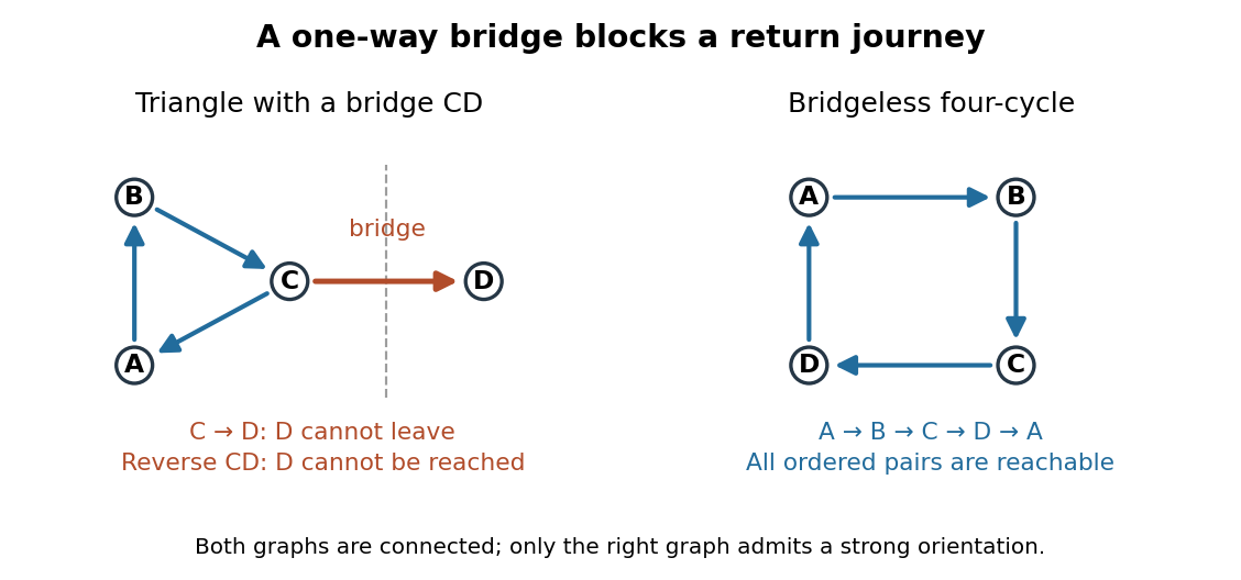
For more than one vertex, a strong orientation cannot also be an acyclic orientation: directed paths from to and back give a nonempty closed directed walk, from which removing repeated portions leaves a directed cycle. A directed graph containing one directed cycle need not have strong connectivity, as the attached shows.
An acyclic orientation is an orientation of a graph whose resulting directed graph has no directed cycle, hence is a directed acyclic graph. A directed cycle must follow every arrow around its closed route. A cycle in a graph in the skeleton of a directed graph only requires the corresponding undirected edges; their arrows need not agree around the route.
For the same triangle in a graph with vertex set and edges , compareBoth have an undirected cycle in a graph in their skeleton of a directed graph. Only has a directed cycle. In , has no outgoing directed edge, so a route cannot continue from back to .
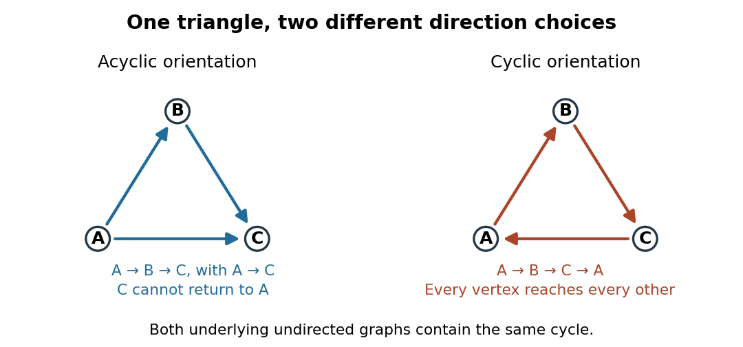
The same triangle in a graph with an acyclic orientation and an orientation of a graph containing a directed cycle
. Details. Thus an acyclic orientation does not require its underlying undirected graph to be a forest. Every orientation of a graph of a forest is acyclic, because a directed cycle would give an undirected cycle in a graph. Conversely, every finite simple graph, including one with many cycles in a graph, admits at least one acyclic orientation by the following ordering construction. On this triangle in a graph, six of the eight orientations of a graph are acyclic; the other two follow the directed cycle in opposite senses.
For a chemical solution in a validated linear regime,where is path length in and is solute mass per final solution volume in . These conventions give specific rotation units . Specify solvent, temperature and wavelength : specific rotation is conditional on the sample environment.[ref]
5.3 Optical Activity. McMurry, Organic Chemistry, §5.3: observed rotation divided by path length and mass concentration
For an original model, stipulate an unnamed enantiomer pair in the same achiral solvent at and wavelength . Assign the positive member specific rotation , assumed constant over the modeled concentrations. With and ,These are chosen model parameters, not measured properties of a named material. Doubling only or only doubles within this stipulated linear model; doubling both multiplies it by four. A real chemical solution must be checked for concentration dependence rather than assuming that is dilute enough.
For an additive mixture containing only this enantiomer pair as solutes, put and write for their mass concentrations. ThenBecause enantiomers have the same molar mass, their relative mole fractions within the pair also equal their relative mass fractions: , . Thus , which connects optical rotation to enantiomeric excess.
Steven Chu's Bell Laboratories team prepared sodium atoms by pulsed-laser evaporation of a pellet. A frequency-swept opposing beam slowed them before six crossed laser beams supplied optical molasses. The vacuum chamber used a shield coated with graphite and cooled with liquid nitrogen as a pump. Fluorescence provided the readout; the initial beams were aligned as closely counterpropagating as possible. [ref]
The manipulation of neutral particles by Steven Chu. Steven Chu, The manipulation of neutral particles, 1998 publication of his Nobel lecture, pp. 687–690, Figs. 3–4 and footnote 5: sodium source, precooling, vacuum apparatus, beam geometry and fluorescence detection
.After equilibration, the team switched off the cooling light for a variable interval, then restored it. Faster atoms escaped during the dark interval; slower atoms were recaptured. The recaptured fraction versus delay constrained the velocity distribution and hence temperature. The inference depended on the initial cloud shape and recapture volume: Steven Chu later acknowledged adjusting a geometry correction towards the expected Doppler cooling limit. Delay was the scanned variable, and the cooling beams themselves supplied the release/recapture control; visible fluorescence alone could not establish temperature. [ref]
The manipulation of neutral particles by Steven Chu. Steven Chu, The manipulation of neutral particles, p. 688, release-and-recapture paragraph: measurement sequence and retrospective account of the geometry correction
.Köhler illumination arranges illumination so that the light source is imaged into an aperture plane while the field diaphragm is imaged onto the specimen. This illuminates the observed field without projecting the lamp's structure into the specimen image.
After focusing the specimen, close the field diaphragm, adjust the condenser height until its edge is sharp, center that image and open it just beyond the viewed field. Separately adjust the condenser aperture to set the illumination cone and the balance between image contrast and optical resolution. Confusing the two diaphragms makes brightness changes difficult to interpret.[ref]
Kohler Illumination Procedure by Duke University. Numbered setup procedure: field-aperture focus, centering and condenser-aperture adjustment
Differential interference contrast microscopy converts small sideways differences of optical path length into visible intensity differences. A polarizer and birefringent prisms produce slightly displaced beams with perpendicular polarizations; after they pass through neighboring specimen positions, the beams are recombined and analyzed so that their relative wave phase controls brightness.[ref]
Specimen Contrast in Optical Microscopy by Nikon Instruments Inc.. Differential interference contrast section and Figure 6: beam shear, recombination and optical-path gradients
For beam displacement small compared with the scale of specimen variation, the phase difference is approximately . Thus a transparent object can appear shaded along the shear direction. Rotating the specimen changes that shading: the relief appearance does not by itself measure three-dimensional shape.
Empty magnification enlarges an image without revealing additional specimen detail. Adequate angular magnification can make existing detail visible to the eye, but it cannot undo the objective's diffraction blur. For equally bright, mutually incoherent optical point sources and an ideal circular optical pupil, a commonly used lateral Rayleigh criterion in object space iswhere is the vacuum wavelength, is the specimen-medium refractive index, and is the admitted half-angle. For this model, and give ; changing only numerical aperture to gives . Changing only the eyepiece leaves this object-space scale unchanged. Illumination, optical coherence, optical aberrations and specimen visibility matter in real instruments; this criterion is not a universal threshold.[ref]
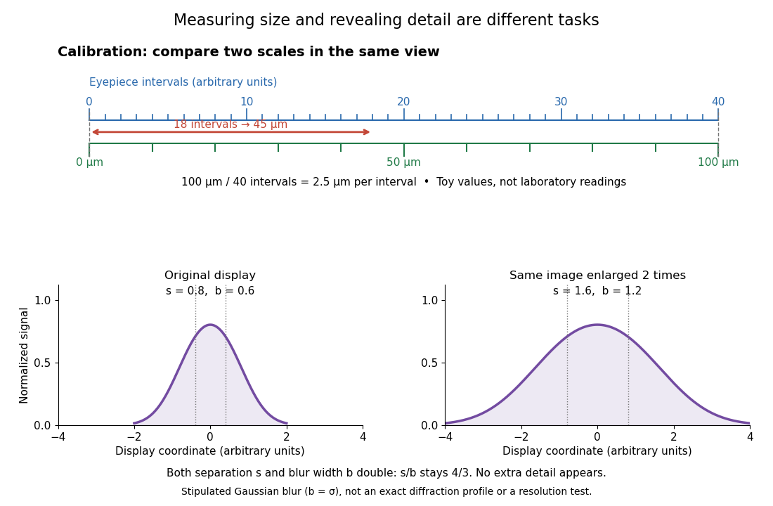
The geometric reason is especially simple. If a fixed recorded image is enlarged by a factor , a feature separation and a blur width become and . Their ratio remainsThis is the lower-panel construction in the diagram. A change to the microscope objective can change numerical aperture and hence the specimen detail captured; a display zoom changes how large that captured detail looks. Microscope scale calibration, diffraction-limited resolution and angular magnification are three complementary properties to report.
Microscope scale calibration compares an image readout with a known specimen length. This documented practical uses an eyepiece graticule, stage micrometer and Köhler illumination. Focus the graticule; place the reference on the stage with the objective-appropriate cover glass. Focus both scales with the chosen microscope objective, then rotate and translate them into parallel alignment. Read widely separated coincidences using consistent line edges. Record the optical configuration and recalibrate for each objective.[ref]
Linear Measurements (Micrometry) by Thomas J. Fellers and Michael W. Davidson. Linear Measurements (Micrometry), Stage Micrometers and Eyepiece Reticle Calibration, Fig. 4 and procedure bullets
The stage micrometer is the reference; preserve the optical configuration when substituting the specimen. Line width, focus, edge selection and optical aberrations limit accuracy. Additional recommended checks are realignment and another known interval: agreement tests repeatability and scale consistency, not absolute reference accuracy.[ref]
Linear Measurements (Micrometry) by Thomas J. Fellers and Michael W. Davidson. Linear Measurements (Micrometry), Conclusions, line-edge choice and calibration errors; repeat-after-realignment check is an additional recommendation
Here is an original toy calculation, not the source's calibration example or measured data. Suppose a reference span coincides with eyepiece intervals. Then the calibration factor and the length corresponding to specimen intervals areThis works because both readouts use the same image-to-specimen scale: . One must count intervals, not tick marks; forty intervals have forty-one bounding ticks. In an ideal linear scale model, if identifying the calibration endpoints introduces a total readout error of interval, the inferred factor ranges from to per interval. Holding exact gives . This isolates one contribution to measurement uncertainty; it is not a complete uncertainty budget or a measured confidence interval.
For a recorded real image, image a stage micrometer at the same capture settings to calibrate length per detector pixel. Resizing changes length per pixel; update the scale bar accordingly. Eye-viewing angular magnification alone supplies no digital image scale.[ref]
Linear Measurements (Micrometry) by Thomas J. Fellers and Michael W. Davidson. Linear Measurements (Micrometry), Conclusions, digital images acquired at identical pixel resolution
An optical microscope whose microscope objective, with the specimen at its designed front focal plane, sends out a parallel bundle of light rays from each specimen point. Different specimen points generally give different bundle directions. A tube lens then forms the finite intermediate microscope image; the microscope eyepiece views it. This parallel region permits suitable optical accessories to be inserted. Finite-conjugate and infinity-corrected components must be matched to their intended system.[ref]
Infinity Optical Systems by Nikon Instruments Inc.. Infinity Optical Systems, Fig. 2(a–b) and following description of objective, tube lens and eyepieces
In the ideal paraxial approximation, an object height at objective focal length gives bundle slope . A tube lens of focal length maps that slope to , soThis is a two-assembly result. Substituting infinity into the single-objective transverse magnification would not describe the finite recorded image. Infinity correction concerns the region after the objective; relaxed-eye viewing concerns the region after the eyepiece. They are distinct conditions.
An optical microscope whose microscope objective is designed to form a real image at a specified finite distance. The intended image distance and optical aberration corrections belong together; mechanical tube length is a mounting specification, not automatically the image distance measured from a principal plane.[ref]
Infinity Optical Systems by Nikon Instruments Inc.. Infinity Optical Systems, opening finite-system discussion and Fig. 2(a)
Why can a small displacement produce a large image? For a converging thin lens, write with . Substitution into the thin lens equation givesThe similar triangles construction supplies the minus sign. The example has and hence . Letting decrease moves the real image farther away; it does not keep the microscope eyepiece in focus at a fixed position. Large transverse magnification therefore requires the correct conjugate geometry, not merely a short focal length.
The real image of the specimen supplied to the microscope eyepiece or a recording surface. In the example above, a bare detector placed at records an image five times the specimen's length, inverted. It does not record a fifty-times image: that number compares viewing angles under the stated reference convention. An optical camera receiving the eyepiece's outgoing light needs its own optical lens to form a further real image, with a recording scale determined by that added image formation.
The viewing optical lens assembly that acts as a magnifier of the intermediate microscope image. With that image at its front focal plane, the outgoing light rays from each point are parallel. In the small-angle approximation, the viewed angle is , versus for the same image-sized object at reference distance , giving .[ref]
A finite-distance virtual image requires a different eyepiece conjugate. In the ideal thin lens model, with the eye close to the eyepiece and the virtual image at distance , the angular magnification becomes . State the viewing condition before multiplying by the objective's transverse magnification; the relaxed-eye example above uses .
The specimen-facing optical lens assembly of an optical microscope. A microscope objective collects light from the specimen and sets the object-side numerical aperture. In a finite-conjugate microscope it forms the intermediate microscope image directly; in an infinity-corrected microscope a tube lens completes that image formation. Its label alone does not calibrate a specimen length.
The optical material surrounding the optical fiber core. In a conventional step-index optical fiber, its lower refractive index permits total internal reflection; it is distinct from the protective coating.
The central guiding region of a conventional optical fiber; in a step-index optical fiber, its refractive index exceeds that of the surrounding optical fiber cladding.
Optical fiber attenuation is the reduction of transmitted optical power along an optical fiber. Define a positive loss in decibels by comparing optical power already launched into the guide with surviving optical power :The factor ten applies to a power ratio; the factor twenty applies to a wave amplitude ratio only when power is proportional to its square under the same conditions.[ref]
Introduction to Optical Fibers, dB, Attenuation and Measurements by Cisco. Introduction to Optical Fibers, dB, Attenuation and Measurements, What is a Decibel?, Base 10 Logarithm Rules and Power/Voltage Gains: attenuation convention
For a uniform illustrative model with constant loss coefficient in and distance in kilometres,For over , the loss is andThus about of the launched optical power survives and is lost. This is an illustrative coefficient, not a property of all optical fibers, and is independent of the earlier illustrative refractive indices.
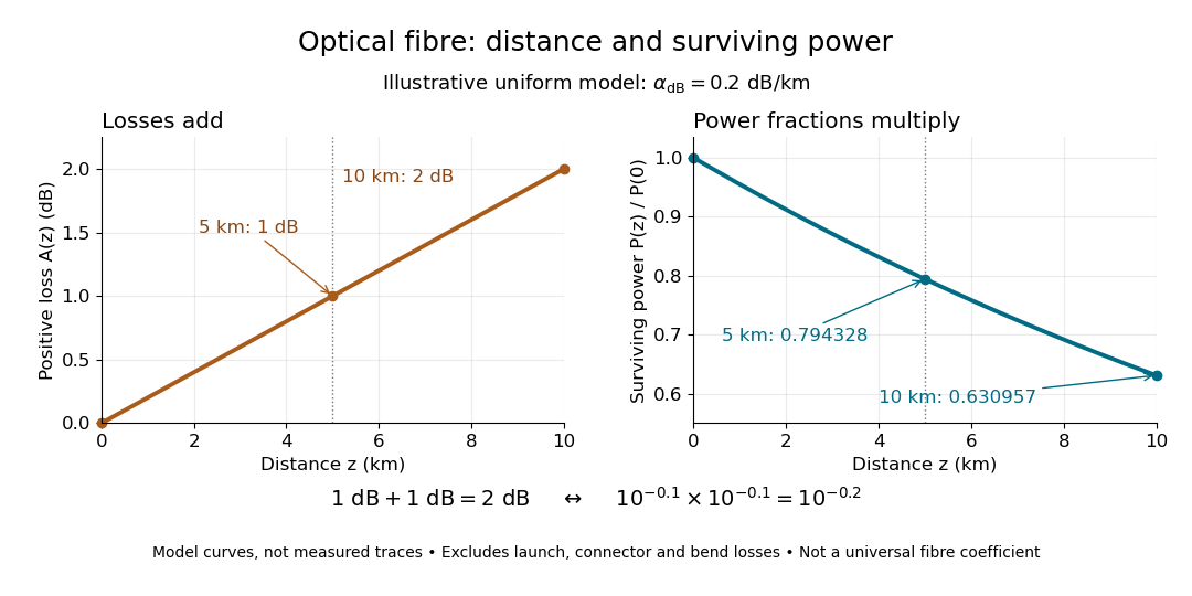
The exponential decay follows from assuming each equal distance interval transmits the same fraction. For two such intervals, power ratios multiply; their logarithms add, so the losses in decibels add. Two sections each transmit ; together they transmit . The loss curve is straight in decibels and curved on a linear power scale.
Wave absorption and scattering of light can remove guided optical power even in a straight fibre, while bends can let it escape. Entrance losses, joints and connectors contribute additional losses; they belong separately from a uniform distance coefficient. This is why a measured end-to-end power ratio need not equal the straight-fibre model.[ref]
Introduction to Optical Fibers, dB, Attenuation and Measurements by Cisco. Introduction to Optical Fibers, dB, Attenuation and Measurements, Understand Insertion Loss and Calculate a Power Budget: joint losses, launch dependence and distance contribution
MIT's Optical Waveguides and Fibers, Laboratory Exercise No. 7 (Fall 2005), describes a teaching apparatus. A cleaned, flat-ended multimode optical fiber receives helium–neon laser light through a microscope objective optical lens; a micropositioner aligns the input. The launch deliberately overfills the fibre's cone. A beam splitter sends a sample to a reference photodetector to track laser fluctuations. The fixed output faces a screen or a photodetector on a rotation stage with angular measurement calibration. Readings every two degrees, divided by simultaneous reference readings, give an angular profile. Repeating with an underfilled launch is a control: too few excited normal modes underestimate numerical aperture. Optional index-matching fluid removes cladding-carried light. Bending the fibre reveals leakage and reduced output on an oscilloscope. The handout supplies no measured trace or absolute detector measurement calibration, and this angular scan does not determine loss per kilometre.[ref]
Optical Waveguides and Fibers (MIT 6.161 laboratory exercise). Optical Waveguides and Fibers, MIT 6.161 Modern Optics Project Laboratory, Fall 2005, Laboratory Exercise No. 7, pp. 3 and 6–7, end-face preparation, §7.3 and Fig. 1: reference-normalized angular scan, underfill control and bend test
A graded-index optical fiber has an optical fiber core whose refractive index varies smoothly with distance from the optical axis. Refraction bends light rays through the varying medium; the straight zigzag of a step-index optical fiber no longer describes their paths. The local launch cone can depend on entry position.[ref]
A single-mode optical fiber supports only its fundamental spatial guided normal mode at the operating wavelength, with possible distinct states of polarization of an electromagnetic wave. The designation must include wavelength: MIT's fibre laboratory explicitly notes that a fibre sold for single-mode operation can support several normal modes at its helium–neon laser wavelength.[ref]
Optical Waveguides and Fibers (MIT 6.161 laboratory exercise). Optical Waveguides and Fibers, MIT 6.161 Modern Optics Project Laboratory, Fall 2005, Laboratory Exercise No. 7, p. 8, §7.4(a): operating-wavelength qualification
Pinned article: Introduction to the OurBigBook Project
Welcome to the OurBigBook Project! Our goal is to create the perfect publishing platform for STEM subjects, and get university-level students to write the best free STEM tutorials ever.
Everyone is welcome to create an account and play with the site: ourbigbook.com/go/register. We belive that students themselves can write amazing tutorials, but teachers are welcome too. You can write about anything you want, it doesn't have to be STEM or even educational. Silly test content is very welcome and you won't be penalized in any way. Just keep it legal!
Intro to OurBigBook
. Source. We have two killer features:
- topics: topics group articles by different users with the same title, e.g. here is the topic for the "Fundamental Theorem of Calculus" ourbigbook.com/go/topic/fundamental-theorem-of-calculusArticles of different users are sorted by upvote within each article page. This feature is a bit like:
- a Wikipedia where each user can have their own version of each article
- a Q&A website like Stack Overflow, where multiple people can give their views on a given topic, and the best ones are sorted by upvote. Except you don't need to wait for someone to ask first, and any topic goes, no matter how narrow or broad
This feature makes it possible for readers to find better explanations of any topic created by other writers. And it allows writers to create an explanation in a place that readers might actually find it.
Figure 1. Screenshot of the "Derivative" topic page. View it live at: ourbigbook.com/go/topic/derivativeVideo 2. OurBigBook Web topics demo. Source. - local editing: you can store all your personal knowledge base content locally in a plaintext markup format that can be edited locally and published either:This way you can be sure that even if OurBigBook.com were to go down one day (which we have no plans to do as it is quite cheap to host!), your content will still be perfectly readable as a static site.
- to OurBigBook.com to get awesome multi-user features like topics and likes
- as HTML files to a static website, which you can host yourself for free on many external providers like GitHub Pages, and remain in full control

Figure 2. You can publish local OurBigBook lightweight markup files to either OurBigBook.com or as a static website.
Figure 3. Visual Studio Code extension installation.
Figure 5. . You can also edit articles on the Web editor without installing anything locally. Video 3. Edit locally and publish demo. Source. This shows editing OurBigBook Markup and publishing it using the Visual Studio Code extension. 
- Infinitely deep tables of contents:




All our software is open source and hosted at: github.com/ourbigbook/ourbigbook
Further documentation can be found at: docs.ourbigbook.com
Feel free to reach our to us for any help or suggestions: docs.ourbigbook.com/#contact