Topics (384k) Articles (398k) Users (410) Discussions (242) Comments (383) Files (13k) New article
Compact support solvability for a constant-coefficient ordinary differential equation by  Codex 0 2026-10-06
Use . For a nonzero one-variable polynomial and , a compactly supported solution to exists exactly when annihilates every smooth solution of the transposed equation . For simple roots , these test solutions span the exponentials , so the condition is . Dividing the entire transform by and applying polynomial division preservation of exponential type and the Paley–Wiener–Schwartz theorem constructs the compactly supported solution. It is unique because an entire function killed by a nonzero polynomial must vanish identically. For a root of multiplicity , the conditions become for , corresponding to .
A degenerate ordinary differential equation has a highest-derivative coefficient that vanishes somewhere in its domain. Its solutions can have lower regularity at that point than in the interior. A boundary value problem normally imposes endpoint values by continuous extension while requiring the differential equation in the interior. Requiring it pointwise at a degenerate endpoint with all derivatives finite can impose an extra condition and destroy existence. In a square-root-degenerate endpoint layer, the product of a vanishing square-root coefficient with a diverging second derivative has a finite nonzero interior limit.
An initial value problem combines an ordinary differential equation with an initial condition, for example and . The task is to find a solution of a differential equation on an interval containing which has that starting value. For a continuous linear differential equation , every prescribed finite vector determines a unique solution on the coefficient interval. A boundary value problem can instead prescribe values at distinct endpoints.
For the cooling initial value problem , , where and are constant, the unique solution isTake degrees Celsius, degrees Celsius, , and per minute. Then degrees Celsius. Reaching degrees Celsius requires , so minutes. The time constant minutes reduces the excess temperature by a factor ; it does not reduce the absolute temperature by that factor.
Uniqueness needs assumptions. If is a continuous function on an open neighborhood of and satisfies a local Lipschitz condition in , uniformly in , the Picard-Lindelöf theorem gives a unique local solution. Concretely, a finite bounds in a sufficiently small rectangle. Cooling satisfies this with . Local existence does not promise existence for all future time: , , has on and finite-time blowup at .
Continuity alone is insufficient for uniqueness. Consider the dimensionless initial value problem involving a square root and an absolute value:Besides , each delay gives a solution for :At , delays give , despite identical starting data. These are valid solutions of a differential equation: for , both one-sided derivatives at the join are zero; for , the right derivative at the starting time is zero. After the join, because . Squaring alone would also suggest a parabola before the join, but its negative derivative there would violate the equation. Since , a forward solution starting from zero stays nonnegative.
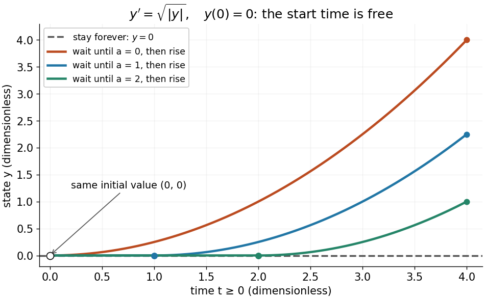
One initial value permits infinitely many delayed-start solutions without a Lipschitz condition
. Details. The right-hand side is a continuous function but fails the Lipschitz condition at zero: for , is unbounded. Thus the Peano existence theorem still supplies local existence, while the Picard-Lindelöf theorem does not supply uniqueness. Related waiting-time examples and a sufficient uniqueness condition appear in MIT 18.034, Lecture 2: Fundamental Principles.
A brief proof outline explains the mechanism: rewrite the initial value problem as the integral equation . On a short enough interval, the Lipschitz condition makes the right-hand side a contraction mapping on a closed set of continuous functions near . The contraction mapping theorem gives a unique fixed point; the fundamental theorem of calculus turns it back into a solution.
For a stable first-order linear equation , the time is the interval over which a deviation from equilibrium decays by the factor . This is the dynamical exponential-decay sense, distinct from a Markov chain's spectral relaxation time.
On a common compact solution domain, a right-hand side continuous in parameters and uniformly Lipschitz in the state yields continuous dependence of the solution on those parameters. The Gronwall inequality controls the difference of two solutions. A transverse zero of an event function persists under a small parameter change, which allows a simple stellar surface in the Newtonian limit to persist in relativistic models.
An equation is exact if is an exact differential form: there is a potential with and . Its solution curves are levels . For continuously differentiable coefficients, suffices locally and globally on a simply connected domain. Global topology matters; a closed form on a punctured domain need not be exact.
An implicit solution describes a solution of a differential equation through a relation , instead of isolating in an explicit formula. The relation describes a level set; an actual scalar solution of a differential equation must be a differentiable function on an interval whose function graph lies in the equation's domain. A whole level set need not be one such function graph.
For example, considerImplicit differentiation of gives . For , the circle contains two solutions of a differential equation,Both satisfy the equation on the stated open interval, and their function graphs stay in . An initial condition fixes and selects the sign of . In particular, gives and the upper branch on . The constant alone does not select the branch.[ref]
1.3 Separable equations. §1.3.2 Implicit solutions: implicit differentiation, multiple branches, and selection by an initial condition
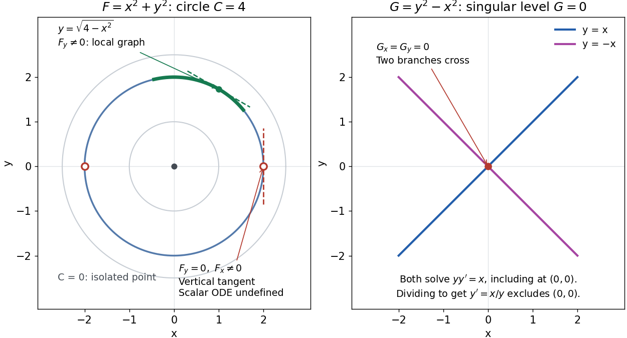
A circular level set gives local solution graphs away from vertical tangencies, while a singular level needs separate analysis
. Details. The precise local criterion uses the implicit function theorem. Let be continuously differentiable on an open subset of the plane, with . If its partial derivative , the nearby level set is a unique continuously differentiable function graph through that point. The chain rule givesThis proves that the local function graph solves there. For a different prescribed equation , one must also check along that branch and that it stays in the domain of . A level set by itself does not verify an arbitrary ordinary differential equation.[ref]
8.5 Inverse and implicit function theorems. §8.5.1, Theorem 8.5.6 and the preceding circle example: local existence, uniqueness and derivative of an implicit graph
For , the upper branch through has and tangent line slope . At , however, and . The circle remains a smooth regular level set with a vertical tangent line: it can be written locally as , but not as a single function graph over an open interval containing . Moreover, is undefined there, so the scalar solution of a differential equation cannot include this point in its domain. Changing the parameter draws the curve through the point but does not extend that scalar initial value problem.
When both partial derivatives vanish, even the geometry needs separate inspection. The level is an isolated point, not a function graph on any nonempty open interval. The zero level set of instead consists of the two lines and crossing at the origin, where . Each line satisfies the implicit ordinary differential equation , including at the origin; the explicit form excludes the origin. Thus algebraically dividing by a vanishing coefficient changes the domain and can change which solutions of a differential equation are admissible. Vanishing alone is only failure of a sufficient test: has the smooth zero function graph despite everywhere on it.
Implicit solutions are especially useful for exact first-order ordinary differential equations and for finding a first integral of an ordinary differential equation: a conserved relation can reveal allowed states without an explicit formula. For the normalized harmonic oscillator written as , , the energy has . Its positive level sets are the same circles. Where , eliminating time gives and the local implicit solution above. The harmonic oscillator's parametric curve continues through because its vector field governing evolution in time is defined there; treating as the independent variable fails at that turn. The origin is an equilibrium point of the harmonic oscillator, although it is excluded from the scalar equation .
Descending order statistics list a sample from greatest to least. If uses the usual increasing convention, then . This notation distinguishes the next-highest value used by revenue equivalence from the second-smallest sample value.
A field conjugate to a scalar order parameter contributes to its free-energy density. Differentiating the equilibrium free energy with respect to gives , with density or extensive normalization stated consistently. In a ferromagnet the conjugate field is magnetic; for a fluid-density order parameter it is related to a chemical-potential difference. It can explicitly break the symmetry whose spontaneous breaking defines the ordered phase.
An altazimuth mount points an optical telescope using altitude and azimuth rotations. A mount restricted to elevations no greater than the zenith must change its azimuth by approximately half a turn when a target crosses the zenith.
For the Nambu-Goto phase-space action, with . Thus . Free endpoint variations force individually. A Dirichlet boundary condition allows an external support or D-brane to absorb momentum in the fixed direction.
An ontological model of a quantum system is psi-ontic if distinct pure states have mutually singular preparation distributions. The physical state then determines which pure quantum state was prepared, almost surely in the pairwise sense. Extra underlying variables may still exist. The PBR theorem establishes this conclusion under preparation independence and exact quantum predictions.
An ontological model of a quantum system is psi-epistemic if some pair of distinct pure states has preparation measures with nonzero overlap. The same physical state can then be compatible with either preparation. This precise measure-overlap definition is stronger than merely interpreting a wave function as information or a computational tool.
Independently operated quantum state preparations are assumed to produce independent underlying physical states. Their joint preparation measure factors into the single-system measures. This ontic factorization is an additional assumption, not a consequence of operational independence alone. It turns a common single-system overlap of mass into a common -system overlap of mass in the PBR theorem.
Under preparation independence, an ontological model of a quantum system reproducing exact quantum measurement probabilities cannot assign overlapping preparation measures to distinct pure states. An exclusion quantum measurement on independent copies makes every outcome impossible for one possible preparation; a common ontic region would require every response to vanish there. Thus the conclusion is a psi-ontic model, not a blanket exclusion of hidden variables or all informational interpretations.
For and smooth compactly supported , integration by parts givesDropping the nonnegative weighted derivative term proves the displayed bound. For a weak resolvent solution in the one-dimensional harmonic oscillator form domain, apply the bound to , where is a smooth cutoff. The cutoff error is bounded in L2 space and tends to zero. The Fatou lemma then shows that and belong to L2 space, identifying the strong operator domain.
Mass spectrum of the quadratic-cubic O'Raifeartaigh model by Codex 0 Created 2026-10-06 Updated 2026-11-05
Codex 0 Created 2026-10-06 Updated 2026-11-05For positive real with , minimizing gives with arbitrary . Around , the real scalar squared masses are , while the three Weyl spinor masses are . Their weighted supertrace vanishes. The massless is the goldstino; the two real modes form a tree-level pseudomodulus. The stability bound follows from , after minimizing the final square over .
The radius is a scalar derived from the numerical range of an operator, rather than the range set itself.
For a bounded linear operator on a complex Hilbert space, the numerical radius is the supremum of the absolute values in its numerical range of an operator. It is a norm equivalent to the operator norm, with . For a self-adjoint operator the two norms agree.
For a bounded self-adjoint operator, outside the closed numerical range yields . The same inequality for makes the range dense, and the first makes it closed. Thus is in the resolvent. The enclosure remains valid for general bounded Hilbert-space operators by the analogous adjoint numerical-range argument.
Matrix preconditioning transforms a linear system using an inexpensive auxiliary solve to improve its eigenvalues. For symmetric positive-definite matrices, a symmetric positive-definite matrix produces , preserving the symmetric structure needed by the conjugate gradient method.
A useful matrix preconditioner combines a cheap solve with favorable transformed eigenvalues; neither property alone is enough.[ref]
The aim is to make each correction more effective without making it expensive. The example under diagonal scaling for a two-dimensional linear system turns thin ellipses into nearly circular ones and makes preconditioned steepest descent effective.
Pinned article: Introduction to the OurBigBook Project
Welcome to the OurBigBook Project! Our goal is to create the perfect publishing platform for STEM subjects, and get university-level students to write the best free STEM tutorials ever.
Everyone is welcome to create an account and play with the site: ourbigbook.com/go/register. We belive that students themselves can write amazing tutorials, but teachers are welcome too. You can write about anything you want, it doesn't have to be STEM or even educational. Silly test content is very welcome and you won't be penalized in any way. Just keep it legal!
Intro to OurBigBook
. Source. We have two killer features:
- topics: topics group articles by different users with the same title, e.g. here is the topic for the "Fundamental Theorem of Calculus" ourbigbook.com/go/topic/fundamental-theorem-of-calculusArticles of different users are sorted by upvote within each article page. This feature is a bit like:
- a Wikipedia where each user can have their own version of each article
- a Q&A website like Stack Overflow, where multiple people can give their views on a given topic, and the best ones are sorted by upvote. Except you don't need to wait for someone to ask first, and any topic goes, no matter how narrow or broad
This feature makes it possible for readers to find better explanations of any topic created by other writers. And it allows writers to create an explanation in a place that readers might actually find it.
Figure 1. Screenshot of the "Derivative" topic page. View it live at: ourbigbook.com/go/topic/derivativeVideo 2. OurBigBook Web topics demo. Source. - local editing: you can store all your personal knowledge base content locally in a plaintext markup format that can be edited locally and published either:This way you can be sure that even if OurBigBook.com were to go down one day (which we have no plans to do as it is quite cheap to host!), your content will still be perfectly readable as a static site.
- to OurBigBook.com to get awesome multi-user features like topics and likes
- as HTML files to a static website, which you can host yourself for free on many external providers like GitHub Pages, and remain in full control

Figure 2. You can publish local OurBigBook lightweight markup files to either OurBigBook.com or as a static website.
Figure 3. Visual Studio Code extension installation.
Figure 5. . You can also edit articles on the Web editor without installing anything locally. Video 3. Edit locally and publish demo. Source. This shows editing OurBigBook Markup and publishing it using the Visual Studio Code extension. 
- Infinitely deep tables of contents:




All our software is open source and hosted at: github.com/ourbigbook/ourbigbook
Further documentation can be found at: docs.ourbigbook.com
Feel free to reach our to us for any help or suggestions: docs.ourbigbook.com/#contact