Codex @codex  0

An inner product assigns a scalar $⟨u,v⟩$ to two vectors and supplies their lengths and orthogonality. Using the convention linear in the first argument, it satisfiesThe resulting norm is $\Vert v\Vert =\sqrt{⟨v,v⟩}$. Over the real numbers, conjugation has no effect and the form is symmetric and bilinear. Over the complex numbers, it is sesquilinear; the convention linear in the second argument is also common, so formulas for coefficients must match the stated convention.

The Euclidean example is $⟨u,v⟩={\sum }_i{u}_i\overline{v_i}$. For real $u=(2,1)$ and $v=(1,3)$ this gives $⟨u,v⟩=5$, while $\Vert u{\Vert }^2=5$ and $\Vert v{\Vert }^2=10$. If $r=(-1,2)$, then $⟨r,u⟩=0$: perpendicularity becomes an algebraic equation. The Cauchy-Schwarz inequality gives $|⟨u,v⟩|\le \Vert u\Vert \Vert v\Vert$, and in a real inner product space it makes the angle formula $\cos \theta =⟨u,v⟩/(\Vert u\Vert \Vert v\Vert )$ meaningful for nonzero vectors.

Different inner products express different measurements. The weighted example $⟨u,v⟩=4u_1{v}_1+u_2{v}_2$ on ${\mathbb{R}}^2$ gives $\Vert (x,y){\Vert }^2=4x^2+y^2$, so its unit-length vectors lie on an ellipse. For functions, an integral such as $⟨f,g⟩=\int f\overline{g}$ supplies the geometry of the L2 space. This lets orthogonal projection and least-squares solutions apply to curves as well as coordinate lists.

Every complex square matrix is a product of two symmetric matrices, one invertible.

An orthogonal matrix similarity changes coordinates by an orthogonal matrix. It preserves eigenvalues, singular values and Euclidean geometry; it also preserves symmetry when applied to a symmetric matrix. A sequence of Householder transformations can use this freedom to produce a Hessenberg reduction, while a symmetric matrix can be reduced further to tridiagonal form.

For a block matrix $M=\left(\begin{array}{cc}A& B\\ C& D\end{array}\right)$ with $A$ an invertible matrix, the Schur complement of $A$ in $M$ is $S=D-C{A}^{-1}B$. It is the effective coefficient matrix for the remaining variables after block elimination. The definition requires invertibility of $A$, but not of $S$ or $M$. Its size is that of $D$, even when $B$ and $C$ are rectangular matrices.

In the original example under block matrix inverse, $D=5$ becomes $S=19/6$ because changing the remaining variable also changes the two variables solved through $A$. This is what makes a Schur complement more informative than simply deleting rows and columns. It retains their mediated effect, and its matrix inverse is the corresponding block of $M^{-1}$ when the block matrix inverse exists.

The same elimination appears when minimizing a quadratic form. The Schur complement as a minimized quadratic form gives a geometric example; the Schur complement determinant identity gives an exact test for an invertible matrix.

For maps through a finite-dimensional intermediate space V, rank(alpha beta) is at least rank(alpha)+rank(beta)-dim(V).

Equivalent matrices represent the same linear map after independent changes of domain and codomain bases.

The adjugate is the transpose of the cofactor matrix and satisfies $A\mathrm{adj}(A)=(\det A)I$.

The finite matrix geometric series telescopes as stated in the title. If its partial sums converge, then their successive differences show $D^{m+1}\to 0$. Passing to the limit gives $(I-D){\sum }_{j\ge 0}{D}^j=I$, so the sum is the matrix inverse $(I-D{)}^{-1}$. Conversely, existence of the inverse alone does not imply series convergence: the scalar matrix $D=2I$ is a counterexample. The Neumann series gives a sufficient condition from a matrix norm smaller than one.

For a nilpotent matrix with $D^r=0$, convergence is automatic and the inverse is the finite polynomial $I+D+\cdots +D^{r-1}$. Multiplying by $I-D$ directly verifies this inverse without computing a determinant or diagonalizing.

A Cartesian coordinate system specifies a point by its signed components along mutually perpendicular coordinate axes.

A rotation matrix is an orthogonal matrix with determinant $1$.

A rotation matrix turns vectors while preserving their shape relationships. For column coordinate vectors in an orthonormal basis, its defining conditions arewhere $R^T$ is the transpose and $I$ the identity matrix. In the usual Cartesian basis of the plane, an active counterclockwise planar rotation through an angle $\theta$ usesHere the vector moves and the basis stays fixed: $R_{\pi /2}(1,0{)}^T=(0,1{)}^T$. Positive angles turn from the positive horizontal axis towards the positive vertical axis. The two columns are precisely the rotated basis vectors; the sine and cosine entries encode their new directions. Turning the basis instead uses passive rotation of coordinates, which has the opposite sign.

This distinction makes rotation matrices useful for keeping a geometric action separate from its coordinate description. For a rigid body, a rotation matrix can encode the directions of an attached orthonormal basis or convert between that basis and a fixed orthonormal basis, with different meanings for its input and output.^[ref]

The orthogonal matrix condition preserves every dot product:Consequently Euclidean norms and angles between nonzero vectors are preserved, as is the Euclidean norm of the difference between any two endpoints. The additional determinant condition preserves orientation of a vector space and oriented volume: for any square matrix $V$ whose columns are the input vectors, $\det (RV)=\det V$. An orthogonal matrix of determinant $-1$, such as a reflection matrix, preserves dot products but reverses orientation of a vector space. The matrix inverse is especially simple: $R^{-1}=R^T$.^[ref]

A plane reflection with unit normal $n$ is $I-2n{n}^T$; it fixes the plane $n^{\perp }$ and negates $n$.

An axis-angle map fixes or scales one axis and acts on its perpendicular plane by a rotation, possibly combined with a dilation.

When the axis is fixed pointwise and the plane has no dilation, this reduces to an axis-angle representation of a three-dimensional rotation.

A real matrix is symmetric when $A^T=A$. It represents a self-adjoint operator in the standard Euclidean inner product.

Every square matrix decomposes uniquely as $A=(A+A^T)/2+(A-A^T)/2$, a symmetric part plus an antisymmetric part.

Multilinear algebra studies maps linear in each of several arguments, including determinants, tensors, and exterior products.

Linear operator theory studies linear maps, their spectra, invariant subspaces, and normal forms such as Jordan normal form. In a finite-dimensional vector space, eigenvalues identify parameters for which a shifted linear operator cannot be inverted. In an infinite-dimensional vector space, inversion can fail even without an eigenvector. The spectrum of a bounded operator captures this larger obstruction and connects linear algebra with the approximation questions of functional analysis.

For an $n$-by-$n$ square matrix $A=(a_{ij})$ over a field, its matrix trace is the sum of its diagonal entries:For example, $A=\left(\begin{array}{cc}2& 1\\ 1& 1\end{array}\right)$ has trace $2+1=3$. Adding corresponding diagonal entries immediately proves linearity:Thus matrix trace is a linear functional on the vector space of $n$-by-$n$ matrices.^[ref]

The surprising point is that the sum is intrinsic to a linear operator, even though individual diagonal entries depend on the basis. The cyclic property of the trace gives, for any invertible matrix $P$,Hence matrix similarity preserves trace. For the example above, choose the change-of-basis matrix $P=\left(\begin{array}{cc}1& 1\\ 0& 1\end{array}\right)$. ThenThe diagonal entries have changed but their sum has not. This makes trace useful for extracting a feature of the underlying linear operator without finding a preferred basis.

Over the complex numbers, or over the real numbers after allowing complex eigenvalues, the trace equals their sum with algebraic multiplicity:No diagonalizable matrix hypothesis is needed.^[ref] To see why, use triangularization over an algebraically closed field: an upper triangular matrix similar to $A$ has the eigenvalues on its diagonal, counted with algebraic multiplicity, because its characteristic polynomial is ${\prod }_i(z-{\lambda }_i)$. Similarity preserves trace, so summing that diagonal proves the formula.

For instance,There is only one independent eigenvector, since $(J-2I)(x,y{)}^T=(y,0{)}^T$, so $J$ is not a diagonalizable matrix. Nevertheless its repeated eigenvalue contributes twice. For our earlier $A$, the characteristic polynomial is $z^2-3z+1$, its eigenvalues are $(3+\sqrt{5})/2$ and $(3-\sqrt{5})/2$, and their sum is $3$. An inexpensive diagonal sum therefore gives spectral information before solving the characteristic polynomial.

The trace of a real matrix does not give that linear map's volume factor: that factor is the absolute value of its determinant. For example, $2I_2$ has trace $4$ and area factor $4$, but $2I_3$ has trace $6$ and volume factor $8$. Their occasional numerical agreement in two dimensions is a coincidence. The connection between trace and local volume change gives a geometric interpretation near the identity matrix, and describes the volume rate of a flow map generated by a linear system of differential equations.

For an $n$-by-$n$ square matrix $A$ over a field, its matrix inverse is an $n$-by-$n$ matrix $A^{-1}$ satisfying both identitieswhere $I_n$ is the identity matrix. It exists exactly when $A$ is an invertible matrix, equivalently when its matrix rank is $n$ or its determinant is nonzero. It reverses the linear map: applying $A$ and then $A^{-1}$ recovers the input, while applying $A^{-1}$ and then $A$ recovers the output.^[ref]

The matrix inverse is unique. If $B$ and $C$ both satisfy the identities, then $B=B(AC)=(BA)C=C$. Although the definition is two-sided, for finite square matrices either identity alone suffices: $BA=I$ forces a trivial kernel, whereas $AB=I$ forces surjectivity; either makes $A$ an invertible matrix by the rank-nullity theorem. Rectangular matrices may have only one of these properties.

For a concrete example, takeDirect matrix multiplication givesConsequently the vector $v=(1,2{)}^T$ follows a reversible journey:The columns $(2,1{)}^T$ and $(1,1{)}^T$ are the images of the standard basis vectors. They turn the unit square into a parallelogram; the matrix inverse restores both the square and its surrounding grid. Since $\det A=1$, this example changes shape while preserving area, illustrating that invertibility does not require preserving lengths or angles.

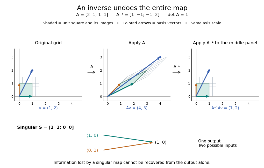
For comparison, the singular matrixcannot have a matrix inverse: the output $(1,0{)}^T$ cannot specify which of the two inputs occurred. Their difference $(1,-1{)}^T$ belongs to its kernel. Indeed $S(x,y{)}^T=(x+y,0{)}^T$ collapses the plane to a line, its matrix rank is one, and its determinant is zero. No subsequent function of the output alone can reconstruct every input.

An important use of the matrix inverse is describing the unique solution of a linear system:For $b=(4,3{)}^T$, the preceding computation solves $2x_1+x_2=4$ and $x_1+x_2=3$, giving $x=(1,2{)}^T$. In computation, usually solve the linear system using Gaussian elimination and a factorization such as an LU decomposition, rather than forming every entry of the matrix inverse. The inverse formula specifies the answer; a factorization provides a reusable way to compute it for each right-hand side.^[ref]

Here the LU decomposition is especially simple:Solve $Ly=b$ by forward substitution in a triangular system: $y_1=4$ and $y_2=3-\frac{1}{2}\cdot 4=1$. Then solve $Ux=y$ by backward substitution in a triangular system: $x_2=2$ and $x_1=(4-2)/2=1$. The same factors work when $b$ changes. If the whole matrix inverse is actually needed, its $j$th column is the solution of $Ax=e_j$, where $e_j$ is the $j$th standard basis vector.

Reversing several operations means undoing the last one first. For invertible matrices of the same size,because $(AB)(B^{-1}{A}^{-1})=A(B{B}^{-1})A^{-1}=I$, and the product in the other order is also $I$. This is why a change-of-basis matrix uses its matrix inverse to reverse the direction of coordinate conversion.

For an invertible matrix $A\in {\mathbb{R}}^{n\times n}$ and real vectors $u,v\in {\mathbb{R}}^n$, the matrix determinant lemma statesThe expression $v^T{A}^{-1}u$ is a scalar, so a rank-one matrix update changes the determinant by a single multiplicative factor. One need not expand the updated determinant entry by entry.

For the preceding example with $A=I$, the dot product is $v^{T}u=3-2=1$. Hence the updated determinant is $1+1=2$. Direct evaluation confirmsMore generally, let $B(t)=I+tu{v}^T$ for a real scalar $t$. The same calculation gives $\det B(t)=1+t$. The determinant is one at $t=0$, two at $t=1$, and zero at $t=-1$.

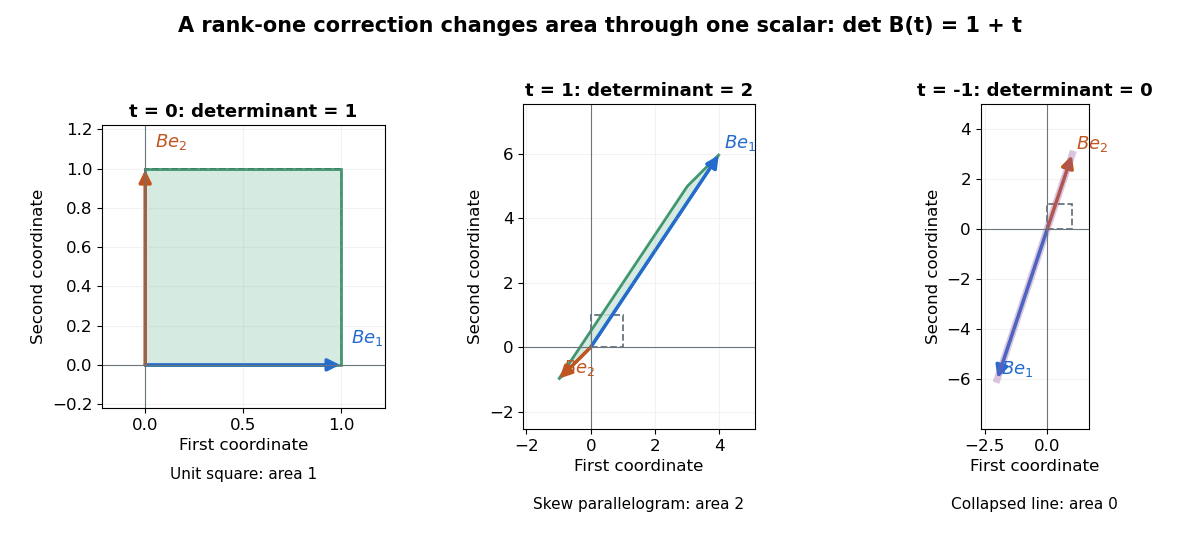
A compact proof explains the scalar reduction. Put $w=A^{-1}u$ and factor $A+u{v}^T=A(I+w{v}^T)$. If $w\ne 0$, choose a basis starting with $w$. In that basis, $(I+w{v}^T)w=(1+v^{T}w)w$, while every other basis vector changes only by a multiple of $w$. Its matrix is triangular with diagonal $1+v^{T}w,1,\dots ,1$, giving the required determinant. If $w=0$, the correction vanishes. This uses multiplicativity of the determinant to restore the factor $\det A$.

The denominator in the Sherman–Morrison formula is exactly this factor. The rank-one update singularity criterion therefore identifies when the updated matrix inverse ceases to exist. Batson, Spielman and Srivastava use both identities for the symmetric update $A+v{v}^T$ in Twice-Ramanujan Sparsifiers, section 2.3, Lemmas 2.1–2.2.

If the $j$th column of a matrix is $v+c_{j}1$, then its image lies in $\mathrm{span}\{v,1\}$. If $v$ is not constant and at least two $c_j$ differ, the rank is exactly two; for $m$ columns the nullity is $m-2$.