
In a linear isotropic dielectric of relative permittivity , the electric displacement field and electric field satisfyHere denotes the free charge density called in the question. For spatially constant , these also give . Equivalently, and . The electric displacement field has units and the electric field has units .
The local equations determine the fields once their geometry and boundary conditions are specified; a density value alone does not determine a unique vector field without that information.
As , the short joining fibre is very stiff and the lower normal mode has . The spheres therefore behave as one torsional load with combined moment of inertia , suspended by the upper fibre of torsion constant . Its angular frequency satisfiesThe high-frequency opposite-twist mode costs increasingly large elastic energy and moves to arbitrarily high frequency in the massless-fibre model.
As , the joining fibre is very compliant. In the higher normal mode the lower sphere scarcely moves: the amplitude ratio tends to . The upper sphere approaches the original single torsion pendulum, givingThe other mode is then a slow twist of the almost freely suspended lower sphere. These interpretations assume the formal limits do not invalidate the thin massless-fibre approximation.
In terms of ,Both curves decrease monotonically: with , , while . The limits, including their leading approach, areThus the limiting squared angular frequencies are and infinity for short joining fibre, and zero and for very long joining fibre. For orientation, at the values are . The high-frequency curve stays above and the low-frequency curve below .
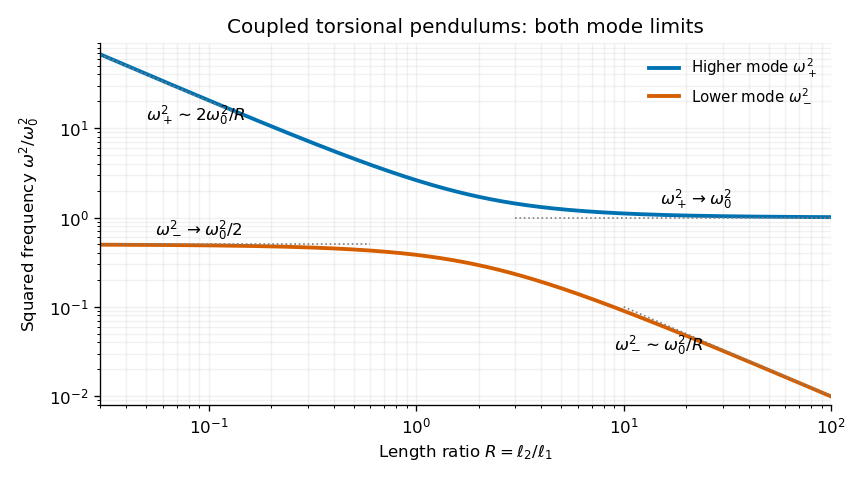
Calculated squared normal-mode frequencies versus fibre-length ratio; both axes are logarithmic to show all four asymptotic limits
. Details. Set and use normal mode amplitudes , with real physical displacements obtained at the end. In units of , the stiffness matrix isWriting , the eigenvalue condition isThereforeFor finite positive fibre lengths both eigenvalues are positive. The corresponding amplitude ratio isThe lower normal mode has the spheres twisting in the same sense, and the higher one has opposite signs of angular displacement.
Let be each sphere's moment of inertia about the fibre, and let be the common fibre filament torsional stiffness, so a length exerts restoring torque . The single-sphere torsion pendulum obeysFor the two coupled torsional pendulums, the upper fibre has twist and the joining fibre has relative twist . The joining fibre exerts equal and opposite torques on the two spheres:Using the measured givesThe fibre's own rotational inertia and damping are neglected, so its twists supply elastic torques without additional dynamic coordinates.
A normal mode of a linearized mechanical system is a motion in which every generalized displacement oscillates at a single common angular frequency, with fixed relative amplitudes and phases. In coordinates , an undamped oscillatory mode may be writtenwhere the amplitude vector is fixed; negative components describe relative phase . An arbitrary small motion is a linear combination of the normal modes when the mode vectors form a complete basis.
At transfer apoapsis, angular momentum conservation givesThe desired circular Kepler orbit has speed . Thusof the original fuel supply is used in the second burn. This is about of the fuel remaining after the first burn. The total transfer consumes of the original supply, leaving about . The two positive impulse magnitudes are added for the fuel budget, even though their directions at opposite ends of the orbit differ.
The original circular Kepler orbit has . For the transfer ellipse, set , in part (c):The first required speed increase is . Under the question's negligible-mass-change fuel model, fuel use is proportional to the magnitude of the impulse. Since the full fuel supply corresponds to ,This is the stated “about a quarter” of the original fuel supply. It is an instance of the Hohmann transfer impulse fractions; no variable-mass rocket model is required under the stipulated assumptions.
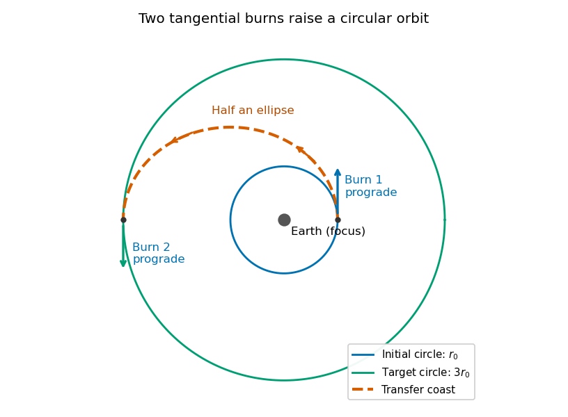
Use a Hohmann transfer orbit. At the initial radius , make a short prograde burn parallel to the existing velocity. The increased speed changes the circular Kepler orbit into an elliptic orbit whose periapsis is the burn point and whose apoapsis lies on the desired larger circle. Coast for half the transfer orbital period to apoapsis.
At that point the transfer velocity is again tangent to the target circle, but its magnitude is smaller than the circular speed there. A second short prograde burn raises it to the required circular speed. Thus both burns increase the instantaneous speed and preserve its direction at the burn, even though the final circular speed is lower than the original one. During the coast the spacecraft loses kinetic energy while gaining gravitational potential energy.


Eliminate using the angular momentum expressions from part (b):HenceFor distinct turning radii, factor the difference of squares and cancel the common factor to obtainThe circular Kepler orbit case is recovered continuously by setting , giving . Combining this with the energy expression also gives for the transfer ellipse.
Choose zero gravitational potential energy at infinite separation. The spacecraft's conserved total orbital energy isAt periapsis and apoapsis, the radial velocity vanishes, so the velocity is perpendicular to the radius. The conserved angular momentum magnitude is thereforeThe angular momentum vector is normal to the fixed orbital plane. The respective units are joules and . These expressions use Newtonian gravity and the approximation .
- Kepler's first law: a bound planetary orbit is an ellipse with the central attracting body at one focus.
- Kepler's second law: the line from that focus to the planet sweeps equal areas in equal times, equivalent to constant areal velocity.
- Kepler's third law: the squared orbital period is proportional to the cube of the semi-major axis, when the orbiting mass is negligible.
The first law includes a circular Kepler orbit as a special case. The third-law constant is the same for bodies orbiting the same dominant mass.
A spatially uniform external gravitational acceleration moves a body's centre of mass without stretching it. Tidal forces arise from the variation of that acceleration across the body. Let a distant mass lie at distance along unit vector , and let denote position relative to the body's centre. Subtract the centre's acceleration. To first order,The tidal tensor is . It stretches along the line to the source with eigenvalue and compresses in the two perpendicular directions with eigenvalues . Its trace vanishes outside the source, consistently with Laplace's equation for the gravitational potential.
After removal of the constant and uniform-acceleration terms, the tidal potential isAn ideal equilibrium ocean on a sphere of radius follows an equipotential of the body's gravity plus this perturbation. For surface gravity , the leading displacement isup to a constant fixing total water volume. The quadrupolar form produces bulges on both the near and far sides; the far-side bulge follows from differential acceleration, without postulating a repulsive gravitational force.
The Moon and Sun both raise terrestrial tides, with relative strength set mainly by , rather than by the total gravitational pull . Their contributions reinforce near new and full Moon to produce spring tides, and partly cancel near quadrature to produce neap tides. Earth's rotation relative to the tidal pattern gives a strong semidiurnal component in the simplest geometry. Real tide heights and timing depend on ocean depth, coastlines, basin resonances, Coriolis acceleration, friction and the declination of the forcing bodies. Tidal dissipation produces phase lags and torques, exchanging rotational and orbital angular momentum and gradually altering the spin and orbit. The equilibrium bulge is therefore a useful starting model, not an exact local tide forecast.
Take a fixed sphere of radius in an unbounded incompressible inviscid fluid, with uniform velocity at infinity. Assume irrotational flow, so and incompressibility gives . Axisymmetry and the dipolar angular dependence of the far field suggestMatching the far field gives . The no-penetration condition then gives . ThusThe surface has stagnation points at its front and rear poles, while the equatorial speed is . Fluid slips tangentially past the sphere; imposing a no-slip condition would contradict this inviscid potential-flow model.
With gravity omitted or the hydrostatic pressure subtracted, steady Bernoulli givesAt the surface,The front–rear symmetry makes the integral of pressure force along the flow vanish: terms proportional to integrate to zero over the sphere. This is D'Alembert's paradox, not a prediction that real spheres have no drag. Viscosity creates boundary layers; separation and a wake break the fore–aft symmetry. Potential flow remains valuable for the outer velocity field when viscous regions are thin, but it cannot supply their drag by itself.
For a slender elastic beam undergoing small bending, cross-sections remain approximately plane and perpendicular to the centreline. At distance from the neutral axis, longitudinal strain is , where is curvature. Linear elasticity gives , so the bending moment has magnitudeHere is the second moment of cross-sectional area, not a mass moment of inertia. For width and depth in the bending direction, . The cubic depth dependence explains why a deep beam resists bending more effectively than the same material spread sideways.
For a uniform beam with transverse displacement , and bending energy is . Balancing transverse load yields the Euler-Bernoulli beam equation under a consistent sign convention. Supports specify values of deflection, slope, moment or shear; the equation alone does not fix the response.
Now apply a compressive end load . A small deflection shortens the axial projection by , so the total potential energy relative to the straight configuration isIts stationary equation isFor pinned ends, and the end moments vanish, so . The candidate shapes require . The first loss of stability is consequentlyAt smaller , the quadratic energy is positive; beyond this threshold the straight configuration no longer minimizes it. End restraint changes the threshold: clamped–clamped gives and clamped–free gives , equivalently an effective-length correction. A column buckles in the direction of smaller flexural rigidity. Euler buckling is a geometric instability within elastic response; yielding or crushing can occur first for a short thick strut. Large deflections, shear deformation and imperfections require refinements of the ideal slender-beam model.
Let the rotating frame have origin acceleration and angular velocity relative to an inertial frame. For a vector referred to the moving axes, the transport rule isApply it twice to position. With rotating-frame velocity and acceleration ,Thus Newton's equation expressed in the rotating frame isThe added terms are translational, Coriolis, Euler and centrifugal fictitious forces. They reflect the frame's acceleration, rather than additional interactions with nearby objects.
The centrifugal force points outward from the rotation axis and, for constant , has potential . The Coriolis force is perpendicular to velocity, so does no work on the particle measured in that rotating frame; it changes direction rather than speed directly. The Euler force is present when the frame's rotation rate or direction changes.
On Earth, gravity and centrifugal acceleration combine into effective gravity. For slow horizontal motion at latitude , the vertical component of Earth's rotation gives Coriolis parameter : an initially northward motion deflects eastward in the northern hemisphere. This supplies a useful local explanation of rotating flows and Foucault precession. A bucket of rotating liquid illustrates the centrifugal potential: its steady free surface is an equipotential of , giving . These equations require a declared frame; adding a centrifugal force while retaining inertial-frame acceleration would count the same kinematic effect twice.
A transmission line must be treated as a distributed circuit when its propagation time is significant on the signal timescale. Let denote resistance, inductance, leakage conductance and capacitance per unit length. Applying Kirchhoff's voltage law and Kirchhoff's current law to a short length gives the telegrapher's equationsFor a lossless line, . Differentiating again gives wave equations withThe travelling solutions can be written and . The minus sign for the backward wave is essential to power transport.
At a load , continuity of voltage and current gives the voltage reflection coefficientA matched termination absorbs the incident signal without reflection. An open circuit has and a short circuit has . Superposed incident and reflected waves produce standing waves. A sinusoidal lossless line of length transforms the termination intofor the convention. At a quarter wavelength, , allowing impedance transformation. A coaxial line supports a transverse electromagnetic mode whose ideal are calculated in A4. Its energy travels in the fields between conductors; the characteristic impedance is not the wire's DC resistance. Losses introduce attenuation and make the characteristic impedance and propagation constant complex.
In a homogeneous Ohmic conductor, . Combining this with Maxwell's equations givesFor a good conductor, , so conduction dominates displacement current. With time dependence and depth , take . ThenThe field is consequently proportional to : it both attenuates and changes phase with depth. The skin depth is the distance for amplitude to fall by ; power density falls as , so its attenuation length is .
Physically, changing fields induce currents whose magnetic field opposes penetration. Equivalently, after neglecting displacement current, magnetic diffusion obeys . Faster changes have less time to diffuse into the metal. Increasing frequency, conductivity or magnetic permeability reduces , provided the relevant material parameters remain applicable.
For a thick conductor the tangential surface electrical impedance is with the stated time convention and consistent field orientation. Its real part represents dissipative resistance per square. Current crowding near the surface raises the AC resistance of a wire when is small compared with its radius; thin strands and laminated magnetic cores reduce suitable eddy-current losses. When , the full complex propagation constant must replace the good-conductor approximation. In a magnetic metal the magnetic permeability can itself be nonlinear and frequency dependent.
Past exam of the physics B course of the University of Cambridge 2019 Paper 2 Section B B6 b Solution Created 2026-10-18 Updated 2026-10-20
A dielectric responds to an electric field mainly by displacing or orienting bound charges, rather than by sustaining a steady conduction current. The polarization density is electric dipole moment per unit volume. It creates bound chargeSeparating these charges from free charge motivatesFor an isotropic linear dielectric, , soThe electric susceptibility describes material polarization and is not the magnetic susceptibility. More generally it is a tensor and can depend on frequency, field strength and temperature.
Electronic polarization displaces an electron cloud relative to its nucleus; ionic polarization displaces positive and negative ions; orientational polarization partially aligns permanent molecular dipoles against thermal disorder. For independent permanent moments of magnitude , weak-field orientational response gives when local-field corrections and interactions are negligible. This explains a common inverse-temperature contribution without asserting that every dielectric follows that law.
At a static interface, and the tangential electric field is continuous. Bound surface charge is already included through . For a homogeneous filled capacitor, , and a reversible linear dielectric stores energy density . At fixed voltage, insertion raises the stored field energy but the voltage source also supplies energy; force arguments must include that source. At fixed charge the capacitor energy instead decreases on insertion.
At frequencies too high for a polarization mechanism to follow the field, its contribution weakens. A complex permittivity represents dissipative dielectric loss as well as phase lag; the sign of its imaginary part depends on the time convention. Strong fields can cause nonlinear response or dielectric breakdown, beyond the reversible linear model.
In a homogeneous linear medium, write and . Without free charge or current, Maxwell's equations becomeTaking the curl of Faraday's law, using , givesTheir plane-wave solutions have and speed ; in vacuum this is . For a wave , the divergence equations give , while Faraday's law gives . Thus the fields and propagation direction form an orthogonal triad, with .
The two independent transverse electric components allow linear, circular and elliptical polarization of an electromagnetic wave. Their relative amplitudes and phase determine the polarization state. In a lossless nondispersive medium the energy density and energy flux areA travelling plane wave has equal electric and magnetic energy contributions and time-averaged intensity , where is its wave impedance and denotes peak electric-field amplitude. Reflection and refraction follow by imposing the electromagnetic boundary conditions. Frequency-dependent constitutive response introduces dispersion; conductivity introduces attenuation, so the simple real constant-speed result has a specified domain of validity.
There are unlisted articles, also show them or only show them.