
Quantum capacitance of a graphene cone 2026-10-18
The quantum capacitance per unit area is . Differentiating the gate equation givesThus the available electronic states act as a second contribution in series with geometric capacitance. At exact neutrality the ideal zero-temperature model has ; actual finite-temperature or spatially nonuniform samples need a broader description. A capacitance measurement can therefore probe the density of states, rather than geometry alone.
Mercury-vapor lamp Created 2026-10-18 Updated 2026-11-05
A mercury-vapor lamp excites Mercury atoms in an electrical discharge and collects the light emitted as they relax. Its output contains characteristic spectral lines; the lamp's pressure and construction affect their widths and the balance between lines and background.
A spectroscope separates those lines, making the lamp useful for wavelength references and optical excitation. Some emitted ultraviolet radiation can excite a phosphor, which converts it into a broader visible output. The observed spectrum then depends on the discharge, envelope transmission and any conversion coating; it is not simply the isolated-atom spectrum at every operating condition.
Vapor Created 2026-10-18 Updated 2026-11-05
A vapor is a substance in a gaseous state at a temperature where a condensed phase can also be reached under suitable pressure conditions. For a pure substance below its liquid-gas critical point, isothermal compression can reach phase coexistence and then convert some vapor to liquid. At coexistence the equilibrium vapor pressure depends on temperature.
A sealed cell containing both water and water vapor illustrates the distinction between amount and state: at fixed temperature, changing the liquid fraction can leave the equilibrium vapor pressure unchanged while both phases remain. A dilute vapor can still approximate an ideal gas, so vapor does not mean that ideal-gas calculations are automatically invalid. Conversely, the broad term gas does not imply ideal behavior. Specifying composition, temperature and pressure makes the usage physically meaningful.
Nuclear gamma-ray multipole selection rules Created 2026-10-18 Updated 2026-10-20
A real photon emitted in gamma decay carries a radiation multipole of integer angular momentum . The triangle rule gives the displayed range. An electric multipole requires , while a magnetic multipole requires . There is no real single-photon decay; an electric monopole transition can instead proceed through internal conversion or, above threshold, pair creation. In the long-wavelength regime , increasing usually strongly suppresses the rate, but nuclear transition matrix elements and collective enhancement can make an allowed lower multipole weaker than a higher one.
Galvanometer readout of an induction pulse Created 2026-10-18 Updated 2026-10-31
A small-angle galvanometer model combines its moment of inertia , damping coefficient and restoring coefficient with a torque per electric current . The resulting damped harmonic oscillator responds to the current pulse through the displayed equation. Its angular deflection can continue after the driving electric current has ceased. Inferring the current's detailed time dependence requires the instrument response, rather than equating needle angle with instantaneous current. This is a generic readout model, not a calibration of Faraday's historical instrument.
Gain narrowing 2026-10-18
Narrowing of a pulse spectrum when the central frequencies receive larger optical gain than its wings. Phase correction alone cannot restore the suppressed spectrum.
Finite-band Cherenkov yield model 2026-10-18
Choose an original transparent-band model, defined only for :This chosen refractive index is not a fit to water, glass or the historical liquids. It decreases from to approximately , so the threshold increases across the band. For , solving givesOnly emits. Faster particles with and emit throughout this chosen band. The Cherenkov cone angle and the Frank-Tamm formula are both evaluated with the same .
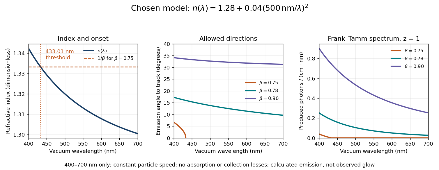
Original dispersive Cherenkov radiation model: a wavelength-dependent threshold, emission angle, and produced photon spectrum
. All curves are calculations for the chosen finite-band refractive index, with and . A missing angular segment means the threshold fails; the corresponding spectral yield is zero. The spectral axis is per centimetre of track and per nanometre of vacuum wavelength, so it is times the density in SI units. No historical observations, measured material constants, absorption or detector response are plotted. Details.
For a track the chosen model predicts about , and emitted photons for , and , respectively. An expected count below one is meaningful over repeated equivalent tracks; it is not a fractional photon observed on one track. The near-threshold example illustrates why extending a constant-index approximation across an entire optical band can give the wrong emitting interval.
Finite bandwidth is essential. The factor cannot be extrapolated down to arbitrarily small wavelength: the chosen material model stops at its stated band. Real optical dispersion changes the threshold and direction, and appreciable absorption requires a complex material response beyond the simple transparent-medium expression. A detected count must also include transport, collection geometry and the detector's wavelength-dependent response. Even a correct produced spectrum therefore does not, on its own, predict perceived colour or observed glow intensity.
Franck-Hertz energy-loss model Created 2026-10-18 Updated 2026-10-20
A useful Franck-Hertz energy-loss model separates three operations: accelerating an electron, losing a discrete energy in an inelastic collision, and selecting the surviving electrons with a retarding collector. The collector measures an accepted fraction of an outgoing energy distribution. This makes the experiment a small inverse problem: the electric current depends on both the collision physics and the readout.
For a deliberately simple one-channel model, let be the incoming kinetic energy, and let be the probability that one encounter excites the chemical atom. Set for and otherwise. The conditional probability distribution of outgoing kinetic energy is the discrete loss kernelHere is the Dirac delta function. The kernel has unit integral, no negative outgoing energy, and mean outgoing kinetic energy . It neglects the small recoil loss in an elastic collision, other excitation channels and ionization. The threshold permits excitation; it does not require above threshold. In particular, choosing a single here isolates the characteristic channel discussed above without claiming it is mercury's lowest possible excitation.
In a dilute thermal helium gas with rapid formation–decay balance of beryllium-8, write its small equilibrium abundance schematically as . A narrow isolated Hoyle state gives a second-step coefficient proportional to . Multiplication yieldswith the stabilizing decay strength absorbed into the coefficient. Here is the Boltzmann constant. The two positive offsets count energy relative to their respective entrance thresholds, not relative to the carbon-12 ground state. A resonance enhances capture at the relevant energy; the Boltzmann factor still selects how many encounters reach it. This is a sequential narrow-level approximation with fixed nuclear widths, excluding plasma screening and changes of composition or mass density.
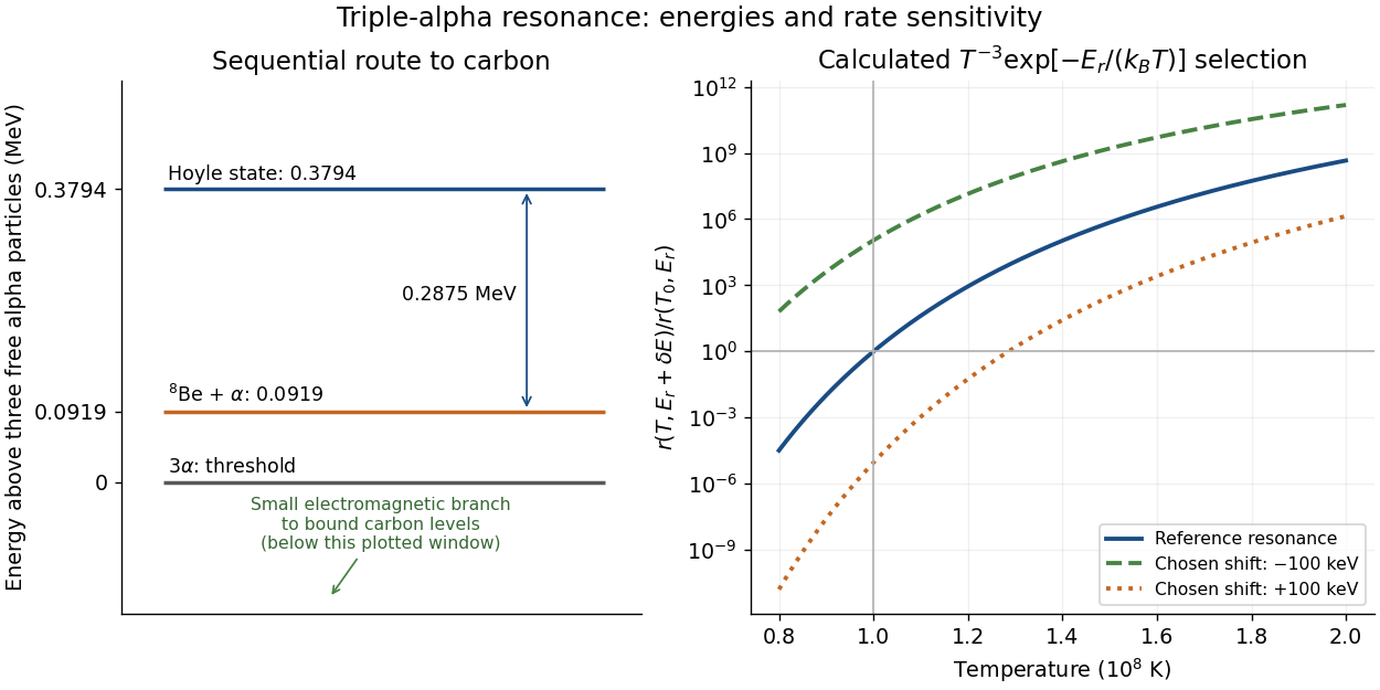
William Alfred Fowler lists the Hoyle state above the carbon-12 ground state, above beryllium-8 plus an alpha particle, and above three alpha particles.[ref]
Experimental and Theoretical Nuclear Astrophysics; the Quest for the Origin of the Elements by William Alfred Fowler. II, p. 179
Subtraction gives for the diagram.Normalize the calculated rate at and . Holding alpha particle number density and the decay strength fixed gives the original sensitivity calculationAt , a deliberately chosen shift multiplies the rate by ; gives . These offsets are hypothetical perturbations, not alternative measured nuclear levels. The reference curve has local temperature exponent of a thermonuclear reaction : raising temperature by gives a factor in this fixed-environment calculation. A real star changes its stellar structure and composition as it burns, so these factors do not directly predict final carbon abundance or a constraint on life.

Laboratory evidence for the Hoyle state 2026-10-18
In 1953, David Noel Ferguson Dunbar and collaborators used accelerated deuterons on nitrogen-14, populating carbon-12 through . Magnetic analysis resolved outgoing alpha particle groups. At incident energy and laboratory angle degrees, they reported excitation , with yield of the group's yield. The stronger group supplied an internal comparison. The paper's opening explicitly relates the search to Fred Hoyle's abundance argument. This is evidence for a nuclear level from a different entrance reaction than stellar fusion.[ref]
The 7.68-Mev state in C12 by David Noel Ferguson Dunbar and others. 1953 paper, p. 649, abstract and opening paragraphs
The inference uses energy and momentum conservation: at fixed incident energy and observation angle, more energy retained as carbon-12 excitation leaves less outgoing kinetic energy. A resolved particle group therefore identifies a nuclear level. This laboratory nuclear line supports an input required by a stellar synthesis model. It does not reproduce core helium burning, measure a complete stellar carbon yield, or by itself determine the stabilizing decay probability.
A Michelson interferometer mirror displacement changes round-trip optical path difference by , giving delay . An interferogram recorded over a finite delay range is multiplied by a window; the recovered spectrum is the true spectrum convolved with that window's Fourier transform. Its characteristic frequency resolution scales inversely with delay range. Consequently a mirror travel range gives and . Numerical width factors depend on the scan definition, window and resolution criterion; the inverse-travel scaling does not.
Interferogram of an equally spaced spectral multiplet Created 2026-10-18 Updated 2026-10-20
For equally intense spectral lines at , sum their delayed self-correlations as a geometric series. The result isThe interferometric visibility revives every . There are zeros between adjacent revivals, at for . The removable singularity at a revival has unit modulus. Revival spacing fixes line spacing; the internal zero count fixes under the equal-intensity model. The interferogram alone does not establish a fixed relative phase between the source lines or prove the emission is a coherent pulse train.
Ising ring magnetization fluctuations 2026-10-18
Define the instantaneous spin magnetization . Global reversal sends to without changing the zero-field energy. Pairing every microstate with its reversed partner proves at every positive temperature, even when almost all probability lies on the two fully aligned patterns. A vanishing mean does not imply weak alignment: the limiting probability distribution is half at and half at .
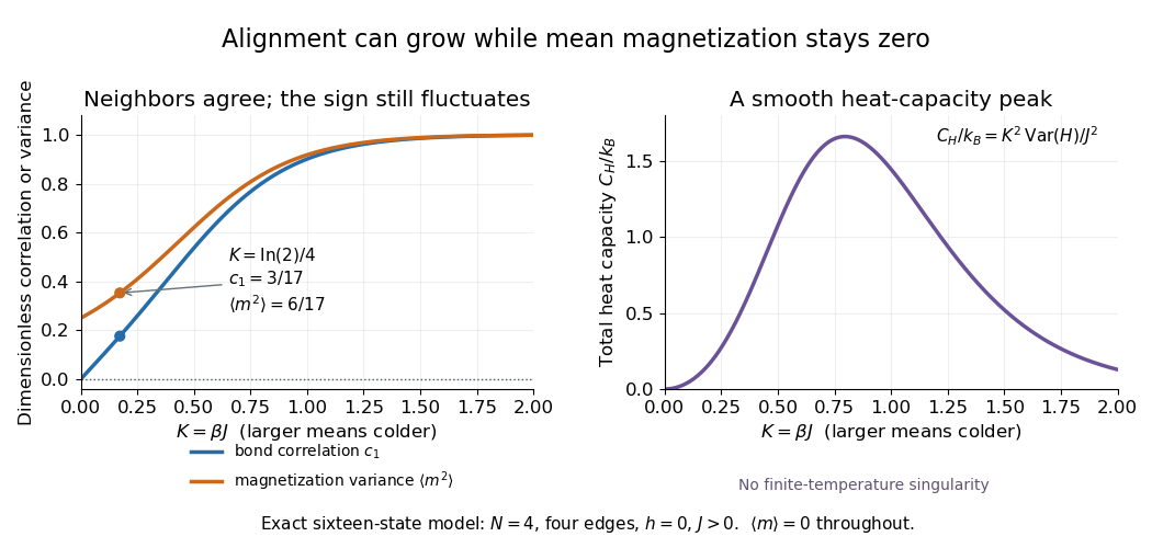
The Ising ring magnetization fluctuations measure this distinction through variance. In the class, both patterns have . Among the patterns, eight have and four have ; the two patterns also have . ConsequentlyIt equals at , approaches for four independent fair Ising spins at , and approaches as . Unlike the energy variance, the spin magnetization variance remains large in the low-temperature symmetric mixture.

The same thermal fluctuation controls the field response. Allow to vary before setting it to zero; differentiating the Boltzmann distribution inserts , givingThis is a spin-normalized magnetic susceptibility with respect to the energy-valued parameter ; conversion to physical magnetization and magnetic field requires the magnetic moment and sample volume factors.
For finite , is a finite positive sum of exponential functions. Its free energy is a real analytic function for , so the smooth heat capacity peak here is not a critical phase transition. Spontaneous magnetization concerns the order of limits: first a thermodynamic limit, then removal of a symmetry-breaking field. The four-spin Ising ring alone establishes neither that limit nor any two-dimensional Ising model result.[ref]
Statistical Physics by David Tong. §5.2.3, paragraph beginning with the analytic finite partition sum: phase transitions require the thermodynamic limit
Ising ring bond correlation 2026-10-18
The Ising ring bond correlation is the neighboring two-point correlation function in the four-spin Ising ring. All four edges are equivalent. At zero field each mean Ising spin is zero by spin inversion symmetry, so also equals the connected correlation function. Agreement gives bond product and disagreement ; thus .
Differentiating the finite partition function with respect to inserts the sum of four bond products. ThereforeHere is internal energy. At , the class-weight calculation gives and . The agreement probability for a selected bond is , despite the exactly zero mean spin magnetization.
A second derivative gives the energy variance, and hence the heat capacity at fixed and :To see the variance identity directly, a derivative of an expected value under weights inserts , where . The factor follows from . At the same exact example, . The heat capacity vanishes both as and as : at high temperature its dimensionless factor vanishes, while at low temperature excited microstates become exponentially rare.
Unique forbidden beta decay 2026-10-18
An th-forbidden beta decay transition with the maximal leading angular-momentum transfer . Only the spin-dependent coupling can attain that transfer at this orbital order. Thus a transition is first-forbidden unique, whereas a same-parity transition is second-forbidden nonunique. Unique refers to the leading weak multipole structure, not a claim that every correction to the decay vanishes.
Immunofluorescence 2026-10-18
Immunofluorescence localizes antigens using antibodies and a fluorescence readout. Indirect labeling uses a secondary antibody to detect the bound primary antibody.
Material volume element Created 2026-10-18 Updated 2026-11-05
A material volume element contains the same fluid particles as it moves and deforms. If its edges transform with the local velocity gradient, its volume changes at a rate equal to the trace of that gradient, giving . Mass conservation states , not that its volume is always fixed. These two identities give the material form of the continuity equation, .
Vertical oscillations of a floating cylinder Created 2026-10-18 Updated 2026-11-05
A vertical cylinder of constant cross-sectional area , partly immersed to depth in a fluid of mass density , satisfies by Archimedes' principle. A small extra downward displacement increases the buoyant force by , so . This is simple harmonic motion with the displayed angular frequency and oscillation period . The ideal model neglects fluid added inertia, drag and surface effects; it requires partial immersion throughout the motion.
Metacentric height 2026-10-18
For a small heel of a floating body in a uniform fluid, the metacentre is the intersection of the new vertical buoyancy line with the original vertical through the centre of buoyancy. With the centre of mass a signed distance above the original centre of buoyancy, the metacentric height is . Here is the waterplane second moment of area about the heel axis and the displaced volume. Positive gives a restoring small-angle torque and negative gives instability. The formula describes local static stability, not all large-angle behaviour or effects of free liquid surfaces inside the body.
Fizeau experiment worked example Created 2026-10-18 Updated 2026-10-25
Choose , , and , with . These are illustrative choices, not measured values or a reconstruction of Hippolyte Fizeau's data. Each beam traverses of water. The nondispersive prediction isThe first number is the offset from rest to one flow setting; the second compares equal opposite settings. The very short equivalent delay explains why interference is useful: a measurable fraction of a wavelength replaces an unattainable direct timing measurement.
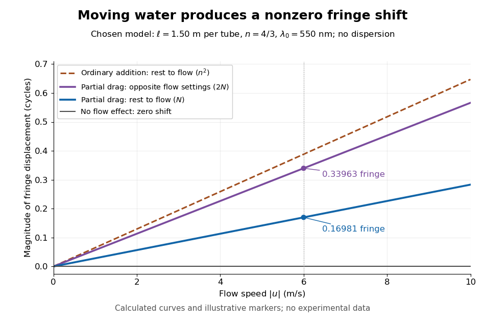
Calculated fringe offsets for chosen parameters: partial drag gives 0.16981 fringe at 6 m/s, whereas equal opposite flows differ by 0.33963 fringe
. Original model curves for tubes of length , refractive index and vacuum wavelength . Solid curves show the first-order rest-to-flow offset and the offset between reversed settings; the dashed curve is the rest-to-flow prediction from ordinary addition of and . No points represent experimental measurements, and optical dispersion is omitted. Details.
The Galilean transformation would give phase velocity magnitudes , hence . At the chosen values this is fringe from rest, larger than the special relativity prediction by . A model with no flow-induced change of phase velocity instead gives . The three alternatives are experimentally distinguishable even when is tiny.
Hippolyte Fizeau's positive displacement favoured Augustin-Jean Fresnel's partial-drag law over zero or full drag. He explicitly distinguished support for that law from establishing its underlying luminiferous aether hypothesis.[ref]
The Hypotheses Relating to the Luminous Aether by Hippolyte Fizeau. Comparison of the three predictions and final paragraph qualifying the inference about Fresnel's hypothesis; scanned translation pp. 572–573
The Fizeau experiment therefore supplies a nonzero relative-motion measurement, not a null test proving an luminiferous aether's absence. The derivation above exhibits the same first-order law within special relativity, showing why agreement with the coefficient alone cannot select an physical interpretation.Two limitations matter for precision. The velocity profile sampled by the beam need not equal the cross-sectional average inferred from volumetric flow rate. Also, the Doppler effect gives opposite rest-frame frequencies for the counterpropagating beams. With optical dispersion, the coefficient in the interference fringe formula becomeswhere the refractive index and its derivative are evaluated for stationary water at the laboratory angular frequency . A wavelength-independent therefore defines an approximation, not a precision fit to real water.[ref]
Fizeau’s “Aether-Drag” Experiment in the Undergraduate Laboratory by Thierry Lahaye and others. Section III, p. 499, equation (7), dispersion from opposite Doppler shifts; section IV.B, pp. 499–500, mean flow versus velocity at the beam
Flow reversal removes a fixed phase difference, but a mechanical or temperature change that reverses with the flow can still imitate the signal and must be controlled. There are unlisted articles, also show them or only show them.