
Ionosphere Created 2026-10-18 Updated 2026-10-20
The ionosphere is a region of the upper atmosphere of Earth with substantial partial ionization. Its mobile electrons and ions constitute a plasma mixed with neutral gas. For radio communication, the crucial question is whether a chosen radio wave returns toward the ground, is absorbed, or passes through. A skywave can connect stations beyond their direct view across the curved surface of Earth, while wave interference between a ground wave and a skywave can make reception fade even when the radio transmitter remains steady.
The ionosphere is useful both as a route for radio communication and as a remote laboratory: varying the probing frequency changes how deeply the radio wave penetrates the plasma. The Appleton-Barnett radio interference experiment turned an unwanted fluctuation in reception into a measurement of the overhead route. Cold-plasma radio dispersion explains why this is a tunable medium, while ionospheric virtual height explains why a measured delay is not automatically an altitude.
Extreme ultraviolet Created 2026-10-18 Updated 2026-11-05
Extreme ultraviolet denotes short-wavelength ultraviolet between longer-wavelength ultraviolet and X-rays; precise band boundaries depend on convention. Its photons have sufficient energy to cause strong optical absorption in many materials that transmit visible light.
This makes beam transport an apparatus problem: an ordinary air path or visible-light window can absorb the beam, and suitable reflective optics can be more useful than an ordinary transmitting optical lens. Before interpreting a weak detector signal, compare a blocked-beam reading with the open-beam reading and account for wavelength-dependent detector quantum efficiency.
Work by Ulf-G. Meißner 2026-10-18
For Cartesian creation and annihilation operators , defineTheir Hermitian adjoints define . The canonical commutation relations imply , with mixed commutators zero. Direct expansion givesEach circular creation adds one energy quantum and angular momentum or . At total occupation , the allowed angular momentum values are , each once in this energy eigenspace.
Tunnel-diode load-line stability 2026-10-18
A current-voltage characteristic determines possible steady operating points; it does not alone determine their linear stability. Consider an ideal voltage source feeding a tunnel diode through a resistor , with a positive constant capacitance across the junction. Assume a quasistatic device relation and neglect inductance, transit delays, noise and heating. Kirchhoff's current law gives the original one-state modelA steady operating point satisfies : the device curve intersects the descending supply line. This is the source-side counterpart of a resistive load line. A small perturbation obeysThus the equilibrium point is locally attracting if and unstable if the inequality reverses. Equality requires higher-order analysis. Even on a negative differential resistance segment, a sufficiently small supply electrical resistance can stabilize this model. The assumption about the electrical circuit matters: an inductive or delayed circuit has additional state variables and may behave differently.
Choose an original toy forward characteristic, with no fitted device parameters:where , and . For every , , so this entire forward curve absorbs positive total power. NeverthelessThe model therefore separates negative differential resistance from negative total . The corresponding peak and valley are at approximately and ; these voltages deliberately differ from the historical peak.
With and , the supply line is . The intersection equation factors exactly:The three operating points are , and . Their values of are respectively , and . The outer two attract nearby trajectories; the middle one repels them. This is bistability in the specified one-state electrical circuit.
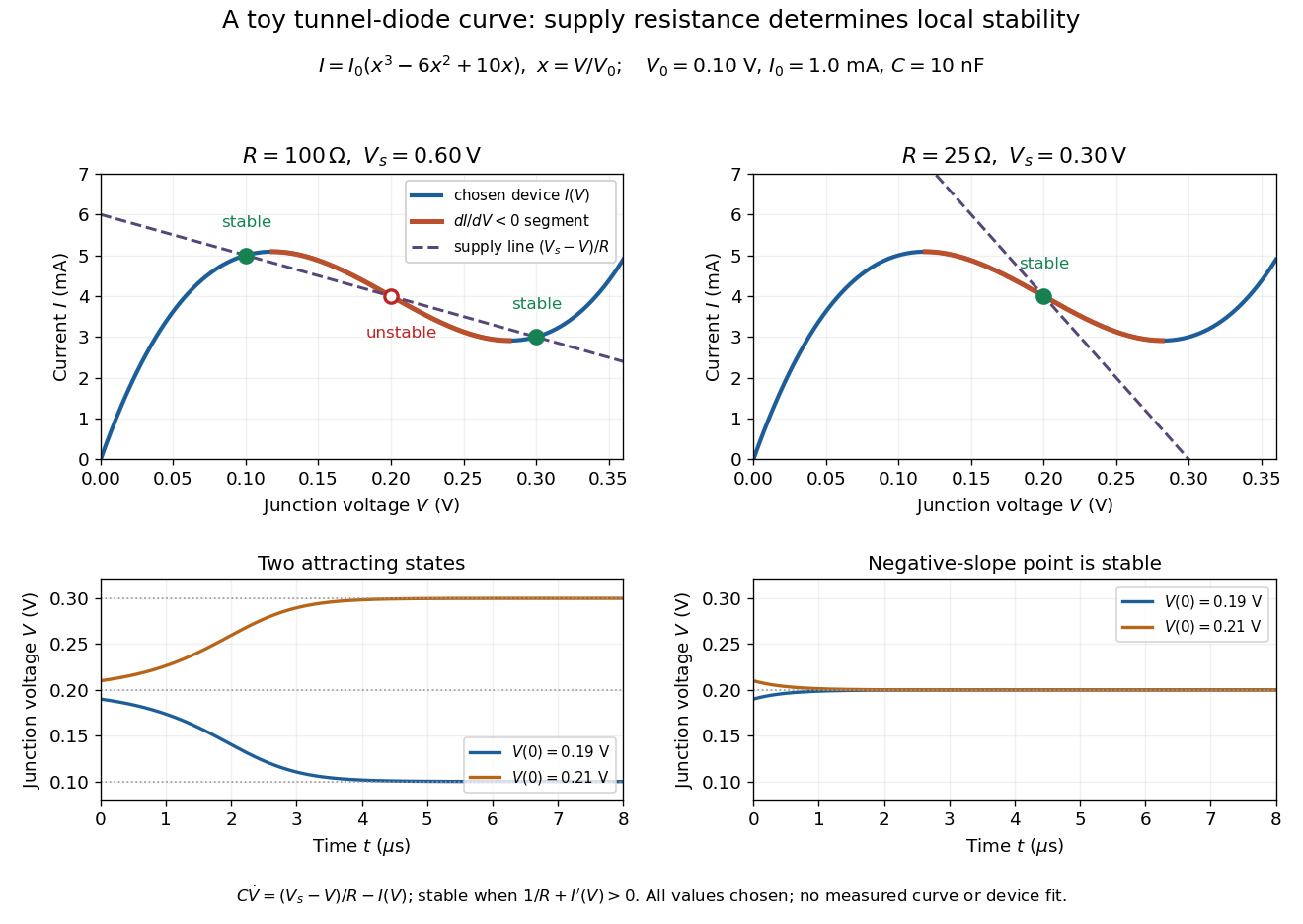

For the second panel, choose and . Now andThere is exactly one real operating point, again . Here , despite the device's own slope . With , the perturbation decays with time constant ; the unstable middle point of the first panel has growth time .
The one-state autonomous model supports switching between attracting operating points after a perturbation or parameter change; it cannot produce a nonconstant periodic orbit. A proposed oscillator needs additional dynamics. This limitation is useful: a load-line intersection establishes a possible steady reading, the slope test establishes local attraction in a specified model, and neither calculation alone predicts an oscillation frequency for a real tunnel diode.
Esaki tunnel-diode experiment Created 2026-10-18 Updated 2026-10-20
Leo Esaki's 1958 report describes alloy-fabricated germanium p-n junctions, with acceptor impurity concentration and donor impurity concentration approximately . Its readout was the current-voltage characteristic: a forward peak occurred at . The report says specimens could be reproduced; above the forward branch approximately followed the ordinary Shockley diode equation.[ref]
New Phenomenon in Narrow Germanium p-n Junctions by Leo Esaki. New Phenomenon in Narrow Germanium p-n Junctions, p. 603, opening paragraph and Fig. 1; opening reproduced on slide 2 of the Trinity College Dublin lecture PDF
In his 1973 lecture, Leo Esaki recalls an earlier junction whose strong room-temperature reverse conduction preceded a negative-slope forward segment revealed by cooling. Its estimated zero-bias width was about ångströms (), supported by capacitance measurements. Increasing semiconductor doping further made the negative slope visible across the measured temperatures, including room temperature. Thus preparation and temperature variation were experimental controls, not merely changes to a theoretical diagram. The low onset voltage argued against avalanche production of electrons and electron holes; the energy band explanation connected the forward decline to loss of available final states.[ref]
Long Journey into Tunneling by Leo Esaki. Long Journey into Tunneling, section II, printed pp. 120–122, Figs. 3–5; inspected institutional mirror at kapitza.ras.ru
The historical readouts were junction electric current versus applied electric potential difference and a separate capacitance check; preparation and temperature were varied. The cited descriptions do not identify a meter model or give a complete wiring diagram.
For a modern repetition, measure junction voltage directly while stepping the supply and recording electric current, repeat both sweep directions, and compare temperatures and differently doped specimens. These are proposed controls, not a reconstruction of the historical apparatus. Lead electrical resistance, Joule heating, contact quality and voltage resolution can obscure the result. The tunnel-diode load-line stability calculation also predicts that an external resistor can make a negative-slope operating point inaccessible in a slow sweep. A jump in terminal readings then need not mean the underlying current-voltage characteristic is discontinuous.
Work by Tsung-Dao Lee 2026-10-18
Missed trypsin cleavage 2026-10-18
Trigonometric identity 2026-10-18
A trigonometric identity is an equality involving trigonometric functions that holds for every input in its stated domain.
Double-angle formula Created 2026-10-18 Updated 2026-10-25
The angle-addition identities give , , and wherever the tangent expressions are defined. The sine formula converts into , which is useful for trigonometric inequalities and integration.
Multiplicity bias from a detector trigger 2026-10-18
A trigger changes which particle populations are common in the recorded sample. Let be the number of particles in an event, and stipulate an independent Bernoulli distribution for each particle's ability to produce an accepted telescope signal, with success probability . If any successful particle suffices, the event acceptance isThis is a deliberately simplified model. Its includes the joint geometrical acceptance and response of the whole telescope; it is not an assumed universal single-counter efficiency. Actual shower directions, spatial correlations and shared electronics can violate the independence assumption.
The conditional probability formula givesFor chosen underlying fractions , and , the two acceptances are and . Five-particle events consequently form about of recorded events. A population that is only of incoming events can occupy nearly of the photographs. This is selection bias, not evidence that the source population changed.
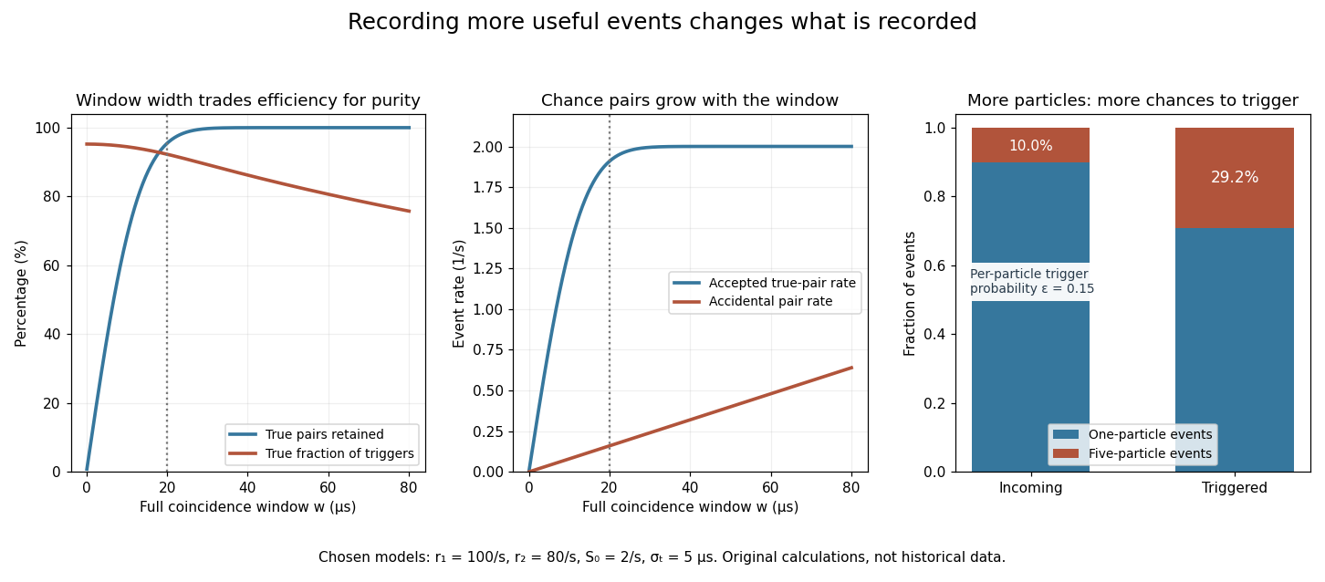
A coincidence window trades timing acceptance against background, while a trigger enriches events with more particles
. Original calculations with the explicitly chosen rates, Gaussian timing spread and independent-particle acceptance model in the text. No historical event counts or measured timing curves are reproduced. Details.
Coincidence circuit 2026-10-18
A coincidence circuit responds when detector signals occur within a specified time window. Two counters placed on opposite sides of a chamber can preferentially select a charged particle that crosses both. Simultaneity within the electronics' window alone does not establish that two signals have the same physical cause: unrelated detections produce accidental coincidences.
Step response Created 2026-10-18 Updated 2026-11-05
The plant output caused by a persistent step change in the plant input, with an explicitly specified initial condition.
Algorithm termination 2026-10-18
Algorithm termination means that execution finishes after finitely many steps on the inputs under consideration. Specify that domain: the stalled loop in partial correctness terminates for but runs forever for . A successful run on one input does not establish termination on another.
A useful method is a loop variant that is a nonnegative integer at every condition check and strictly decreases whenever the condition is true and the body completes. Also prove that condition evaluation and each body execution terminate. An infinite run would then give an infinite strictly decreasing sequence of nonnegative integers, contradicting their well-founded relation. This establishes algorithm termination without enumerating all executions.
For the summation loop verification, begins at and decreases by exactly one per iteration. The body executes exactly times, including zero times for . Merely bounding a decreasing measure below is insufficient for real numbers: decreases forever while staying positive. The choice of a well-founded relation supplies the essential progress argument; well-founded progress in recursion applies the same idea to recursive calls.
Work by Toshihide Maskawa 2026-10-18
Torsion pendulum Created 2026-10-18 Updated 2026-11-05
A torsion pendulum oscillates by twisting a suspension rather than by swinging its support. A horizontal bar suspended from a thin wire experiences an approximately linear restoring torque for small angular twists. With moment of inertia about the wire and negligible damping, its equation of motion and period of an oscillation areHere is the torsion constant, and the angle is measured from the untwisted equilibrium.
Twist the bar gently, release it, and time several complete cycles. Adding two equal masses at equal distances from the wire increases without moving the center of mass off the axis, so the period of an oscillation increases. This makes a torsion pendulum useful for measuring a moment of inertia or calibrating the suspension of a torsion balance.
Discharge measurement in a draining tank 2026-10-18
James F. Price's Draining a Tank, an appendix to Dimensional Analysis of Models and Data Sets, describes an actual tabletop experiment in sections 2.1–2.3. Tap water filled a semitransparent polypropylene beaker with a marked volume scale and drilled side openings. Some trials added horizontal outlet tubes. Temperature was measured, and dye checked that the water had settled before uncovering the outlet. The readout was elapsed time at successive volume marks. Opening diameter and tube length varied between trials. Reported repeatability was checked; tube bores were measured with feeler gauges rather than accepted from nominal sizes.[ref]
For tank area and volume at outlet level, the observations give and interval volumetric flow rate . Price compared across heads to infer a discharge coefficient where that ratio was nearly constant. At small head, drainage could stop with a protruding water cap; surface tension mattered. Outlet tubes introduced viscosity effects. This experiment tests a useful operating range, rather than proving ideal drainage down to zero head.[ref]
A useful independent test of the constant-coefficient model avoids numerical derivatives of noisy head readings. Its exact square root relation predictsFit a straight line to against time over a chosen positive-head interval; the negative slope determines . Repeat from the same initial head and compare slopes, then vary the head interval to test constancy of . This is a proposed diagnostic derived from the draining tank with constant cross-sectional area, not an additional procedure or measured fit attributed to Price. Startup transients, uncertain outlet level, a changing jet shape and terminal low-head data can spoil the straight line. Independent collection of discharged volume provides a check on the tank-scale readout.
Take a reservoir with constant horizontal cross-sectional area , one small orifice of area , no inflow, and constant stipulated discharge coefficient . Let the initial head be . For constant mass density , the stored mass above the outlet level is and outgoing mass flow rate is . Mass conservation cancels and gives the initial value problemThe downward speed of the free surface is , smaller than the ideal jet speed by the factor . Thus a small opening relative to the reservoir supports the negligible-surface-velocity assumption.
For , separation of variables or the chain rule gives . Integrating yieldsThe model reaches zero head in finite time even though volumetric flow rate tends to zero. Extending the squared expression beyond would make head grow again and violate the original ordinary differential equation. The zero-head continuation enforces no further outflow. For an elevated side opening, zero head means the surface has reached that opening, leaving fluid below it; is not the time to remove every drop from such a tank.
For an original synthetic example, stipulateThe initial volume above outlet level is . The initial ideal jet speed is , the initial volumetric flow rate is , and the predicted zero-head time is . These are consequences of stipulated parameters, not experimental measurements. At , head is , stored volume is , and volumetric flow rate is . Half the initial volume has already left at .
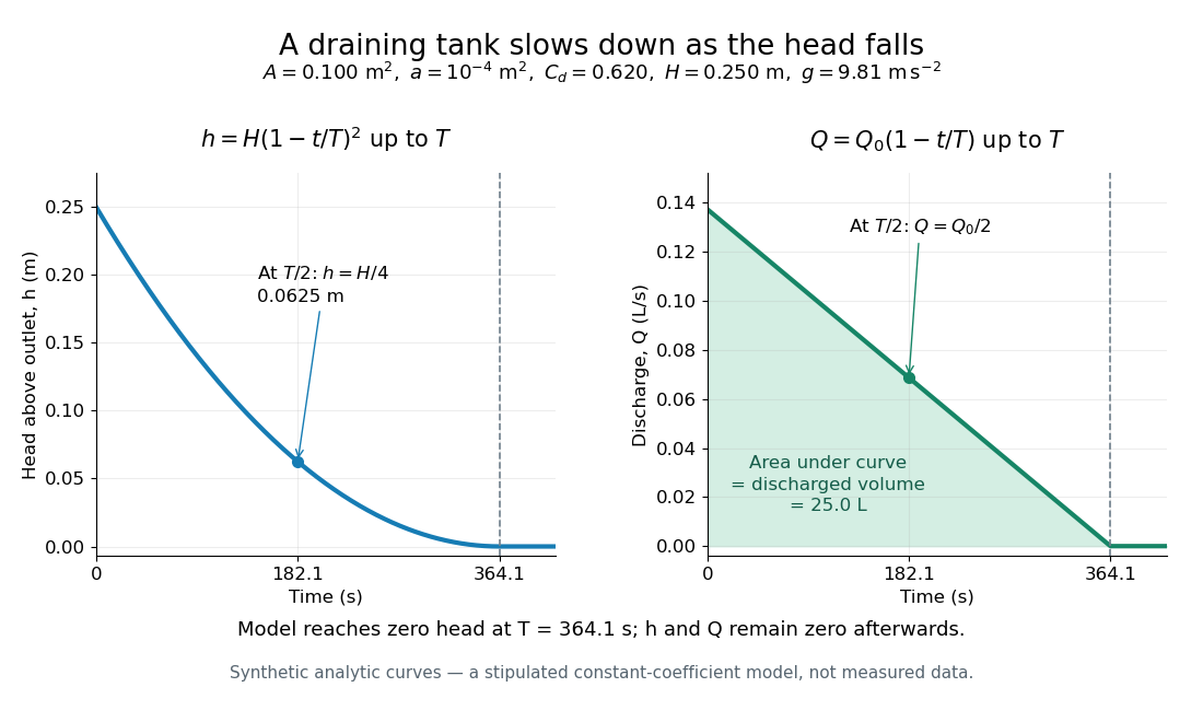
Constant-area drainage: quadratic head and linearly declining discharge
. Original synthetic trajectories for the stipulated draining tank with constant cross-sectional area, with , , , and . The model remains at zero head and zero volumetric flow rate after . The shaded area under the flow curve represents . Details.
An independent mass conservation check integrates the outgoing volumetric flow rate:Multiply both sides by mass density to obtain discharged mass. A dimensional analysis check gives , and . The triangular area under explains why the initial-rate estimate is only half the actual model time. Doubling doubles ; doubling or halves , within the same assumptions.
This finite-time result is an idealized prediction. The constant and quasi-steady approximation need not survive very small head or the initial startup. Appreciable viscosity in a narrow outlet tube requires a different pressure balance, as in Poiseuille flow; appreciable surface tension can prevent zero head altogether.
Haldane conjecture 2026-10-18
For the uniform, nearest-neighbour, isotropic Heisenberg antiferromagnet chain, the Haldane conjecture distinguishes integer spin , with a nonzero bulk excitation spectral gap, from half-odd-integer , with gapless excitations in the thermodynamic limit. The continuum nonlinear sigma model contains a topological angle : integer and half-odd-integer spins give and modulo . This is a different use of topology from the two-dimensional occupied-band Chern number. The chain belongs to the Haldane phase.[ref]
Nobel Lecture: Topological quantum matter by F. Duncan M. Haldane. Haldane, individual Nobel lecture delivered 8 December 2016, published 2017, pp. 040502-8–9: integer versus half-odd-integer chains and topological angle
Chern insulator 2026-10-18
A Chern insulator is a two-dimensional band insulator whose occupied energy bands have a nonzero total Chern number. It has a bulk band gap, yet an interface with a topologically trivial band insulator carries a net excess of quantum Hall edge states propagating in one direction. Time-reversal symmetry must be broken. The Haldane model shows that a nonzero average magnetic flux is unnecessary.
Why distinguish two solids that both have a band gap? The energy eigenvalues tell us whether an excitation costs energy; the energy eigenstates also describe how the state changes around the Brillouin zone. Their Berry curvature can integrate to a nonzero integer. A small deformation changes the Berry curvature continuously, but cannot continuously change an integer. A Chern insulator and a trivial band insulator therefore cannot be connected through a path of isolated occupied energy bands with a common bulk band gap. The distinction survives sufficiently weak local perturbations. It does not make every microscopic quantity or every boundary state immune to every disturbance.
For a single filled energy band, set the Berry connection to , and orient the momentum plane by . ThenThis is the First Chern class evaluated on the Brillouin zone, a torus. Smooth eigenvectors may require multiple patches; their transition phases have integer winding numbers. For charge and conventional electric current , these conventions give and . The measurable magnitude agrees with Chern number and integer Hall conductivity. Reversing the momentum orientation or the sign of the Berry connection reverses the displayed .
There are unlisted articles, also show them or only show them.