
Past exam of the mathematics course of the University of Cambridge 2005 iii Paper 63 7 Solution Created 2026-10-03 Updated 2026-10-14
Geometric quantization. A classical symplectic manifold supplies observables as real functions, their Poisson bracket, and Hamiltonian flows. Geometric quantization seeks a Hilbert space of quantum states and operators that encode this structure, including and a commutator corresponding to the Poisson bracket. A direct prescription cannot make every classical product become an operator product without qualification; operator ordering and the choice of physically admissible observables matter. The aim is to build the state space and operators from the geometry rather than from a preferred coordinate chart.
For prequantization, with , choose a Hermitian line bundle with a unitary connection on a vector bundle of curvatureIts first Chern class requires the integrality conditionEquivalently the symplectic period on every closed integral two-cycle is a multiple of . Conversely an integral class supplies a line bundle, and a unitary connection can be adjusted by a one-form to have the required curvature. Locally choose with ; then . Potentials differing by an exact one-form change the local phase of the section. Integrality is precisely what makes these local descriptions glue consistently.
On sections the Kostant-Souriau prequantum operator isThe curvature identity , together with , givesIndeed the derivative part of the commutator is , the curvature part is , and the two multiplication/derivative cross terms total . These combine to the displayed operator identity. The prequantum inner product uses the Hermitian fiber metric and the symplectic volume form , with appropriate square-integrability and operator-domain conditions.
This is not yet the desired quantum state space: a prequantum section depends on all phase-space variables, whereas a wavefunction normally depends on only configuration variables. A polarization in geometric quantization is an involutive Lagrangian rank- subbundle of . Polarized sections obey along that distribution. The symplectic form vanishes on it, so its restricted curvature vanishes and these differential conditions are locally compatible.
For , the vertical polarization is spanned locally by . With , polarized sections depend only on , and the basic prequantum operators becomeOnly observables whose Hamiltonian flows preserve the polarization act directly on this polarized space. A generic quadratic kinetic energy does not preserve the vertical polarization, so obtaining its quantum operator needs an additional construction rather than simply restricting every prequantum operator. A compatible complex structure can instead provide a Kähler polarization, yielding holomorphic-type states, as for oscillator variables. The Blattner-Kostant-Sternberg pairing compares suitable state spaces of different polarizations and can implement some transported observables.
Finding a useful global polarization is a genuine problem: it may not exist as a nonsingular real foliation; leaf holonomy can obstruct globally nonzero flat sections; singular leaves and compact leaves impose further conditions. A metaplectic correction uses half-forms to improve the inner product and coordinate transformation law and account for familiar zero-point shifts, when its additional square-root data exist. Thus prequantum integrality, polarization, Hilbert-space completion and observable domains are separate steps, each with geometric constraints.
Applications of Stokes's theorem. For an oriented manifold with boundary and a differential form of degree ,with the outward-normal-first boundary orientation. Locally the identity is integration by parts in a half-space; a partition of unity reduces the general manifold to that local calculation, and contributions along internal patch boundaries cancel. The Generalized Stokes theorem unifies the fundamental theorem of calculus, circulation/flux formulas and the relation between local conservation laws and conserved integrated charges.
For a charged brane with worldvolume of dimension , let be its embedding, its induced worldvolume metric, and a -form gauge potential with . TakeUnder , the Wess-Zumino brane coupling changes by . It is invariant for a closed worldvolume, or for suitable boundary conditions; open branes can require compensating boundary terms.
For an embedding variation , differentiation of the pullback and Cartan's magic formula giveThus the interior force depends only on the gauge field strength. In components, define the worldvolume wave-map/mean-curvature vector byVarying the area term and integrating by parts gives . Combining the two variations yields the field-strength force on a charged brane equationIt is gauge invariant because no longer occurs. Its tangential projection vanishes identically by antisymmetry, consistently with worldvolume reparametrization invariance. At , the chosen Lorentzian worldline convention has in proper time and recovers the usual Lorentz-force sign.
For topological conservation, let the spatial manifold compactify to a closed oriented -manifold , and let a field take values in a closed oriented -dimensional target with normalized volume form , . ThenThis is the degree of a map between oriented manifolds: for a regular value it is the signed sum of inverse images. To relate the integral to that count, use a normalized target form supported near a regular value and change variables on its inverse-image neighborhoods. Any two normalized top forms on a connected closed oriented target differ by an exact form, whose pulled-back integral vanishes by the Generalized Stokes theorem. Hence the value is independent of this localization and equals the integer signed count.
If varies smoothly in time, its spacetime pullback satisfies . Apply Stokes theorem to the spacetime slab between two slices: the difference of their charges is minus the flux through the spatial boundary. With no flux at infinity, is conserved independently of the field equations. Equivalently a smooth homotopy cannot change the degree. Singularities, altered boundary conditions or nonzero boundary flux are the ways the argument can fail.
For the Skyrme model, finite-energy fields approach at spatial infinity, so compactifies to and . With the conventional target orientation chooseThis is a normalized closed target volume form. The resulting topological baryon number in the Skyrme model isThe corresponding identically conserved spacetime current is in oriented flat coordinates. For the hedgehog with and , substitution givesThe Skyrmion therefore supplies a concrete topologically conserved unit charge. Topological conservation alone does not guarantee a stable finite-size static solution: the positive Skyrme term, with four derivatives, opposes collapse of the two-derivative energy. Under size rescaling, these contributions behave as and , allowing a nonzero equilibrium size while preserving the degree.
Past exam of the mathematics course of the University of Cambridge 2005 iii Paper 63 6 Solution Created 2026-10-03 Updated 2026-10-14
Use and . For an actual infinitesimal left Lie group action, define . Its fundamental vector fields obey with this convention.
Existence and its global obstruction. Preservation of the symplectic form gives . By Cartan's magic formula, is closed. Locally it equals ; globally this requires its class in to vanish. If it does for every , choose potentials linearly in and defineThis gives the component Hamiltonians of a weakly Hamiltonian action. The assumption in the question does not alone guarantee a global moment map: on with , translation in preserves , but its contraction is , whose integral around the circle is nonzero. It is not an exact one-form. Thus no global real-valued component Hamiltonian exists for that circle action. The intended construction is valid locally, or globally with this exactness condition, for example if .
Matching the Lie algebra. On each connected component, the moment-map equivariance obstruction is the constantIndeed, the identities and show that its differential vanishes. The Jacobi identity for the Poisson bracket saysChanging by a linear constant changes to . Consequently the necessary and sufficient infinitesimal condition is the cocycle must be a coboundary, so that the constants can be chosen withEquivalently its class in vanishes. For a connected group this infinitesimal equivariance integrates to equivariance under its coadjoint action. A disconnected group can impose additional conditions. Here “coincides” means representing the specified Lie brackets; it does not guarantee injectivity when the group action has ineffective generators.
Proof using the Killing form. A nondegenerate Killing form makes semisimple. First, it is perfect: the -orthogonal complement of is the center by invariance, and the center is zero by nondegeneracy. For symplectic fields,by Cartan's magic formula and the antihomomorphism sign. Every commutator therefore has an exact contraction. Perfectness supplies component Hamiltonians for every generator, even when is not simply connected: this is Hamiltonian existence for a semisimple symplectic action.
It remains to eliminate the cocycle, not merely to name an existence theorem. Define a linear operator on by . Antisymmetry of makes skew for . Combining its cocycle identity with invariance of givesChoose by , possible because is nondegenerate. Since is a derivation, . Cyclicity of the matrix trace then givesThus , and . Taking removes , proving the required condition. This applies to semisimple Lie groups, including for , and for . It is nondegeneracy, not positive definiteness, that matters. Groups with a nonzero central Lie algebra, such as , do not satisfy this Killing-form criterion, although particular actions can still have equivariant moment maps.
The isotropic oscillator. On , putThe action , , preserves the Hermitian norm and the symplectic form, and therefore preserves . A Hermitian matrix parametrizes the Lie algebra generator . Its unitary moment map of an isotropic oscillator isSince , direct differentiation yieldsThe matrix is Hermitian and corresponds precisely to ; no central defect remains. The full moment map can be identified, using the pairing with Hermitian matrices, with the rank-one matrix . The central generator gives , whose flow is . Globally , so the “ factor” refers to this central circle, rather than a literal direct-product decomposition.
The real orthogonal subgroup acts geometrically by , the cotangent lift of a diffeomorphism of . If is real antisymmetric and , then . For , this is , so its three components are the usual angular momentum .
The remaining six independent Hermitian directions can be taken as real symmetric matrices. Their moment functions spanThe diagonal ones are the individual oscillator energies; their sum is . The off-diagonal ones correlate two oscillator modes. Their flows mix positions and momenta and are not cotangent lifts of the obvious spatial rotation action: for a real symmetric , and , rather than , . All nine quadratic functions commute with , since the entire unitary group action preserves the oscillator Hamiltonian.
Past exam of the mathematics course of the University of Cambridge 2005 iii Paper 63 5 Solution Created 2026-10-03 Updated 2026-10-14
A symplectic manifold is a smooth manifold with a closed, nondegenerate two-form . Nondegeneracy forces . Examples are with , an oriented surface with a nowhere-zero area form, and every cotangent bundle with its canonical form.
A Poisson manifold has a bivector such that is an antisymmetric bilinear Poisson bracket, is a derivation in each argument, and satisfies the Jacobi identity. Its rank need not be full or constant. The zero bivector gives a Poisson manifold on any smooth manifold, including an odd-dimensional or nonorientable one. A nonzero example on is the Lie-Poisson bracket : it has rank two off the origin and rank zero at the origin, so it does not arise from a symplectic form on the whole three-dimensional space. Even on , is Poisson, since its Jacobi condition is a three-vector and hence vanishes, but its degeneracy on prevents it from being the inverse of a global symplectic form. A manifold carrying a degenerate Poisson structure might separately admit some other symplectic structure; these are distinct claims.
At each point of a symplectic manifold, linear nondegeneracy gives a basis with . Its top wedge product of differential forms isThus is a global nowhere-zero volume form and selects a consistent symplectic orientation. This proves every symplectic manifold is orientable without choosing a global frame.
Let and let a point of the cotangent bundle be with . Define the canonical Liouville one-form intrinsically by . In local coordinates it is , soThis definition is global, by , and its coordinate matrix has invertible blocks. Hence is symplectic for every smooth , even if itself is not orientable.
The coordinate Jacobi condition for a Poisson bivector isNecessity follows by applying the Jacobi identity to three coordinate functions. For arbitrary functions, the second-derivative terms in the Jacobiator cancel by antisymmetry of ; the terms left are exactly this coefficient multiplying , proving sufficiency.
For a symplectic form, take and . With these signs the matrix of is . Differentiation gives . The cyclic expression above consequently equalswhich vanishes because . This directly proves that a symplectic manifold defines a Poisson manifold.
Past exam of the mathematics course of the University of Cambridge 2005 iii Paper 63 4 Solution Created 2026-10-03 Updated 2026-10-14
Use the convention , with . Expanding the Jacobi identity on three basis elements givesso each coefficient satisfiesAntisymmetry in the input indices makes this equivalent toThe vertical bars exclude the summed index from antisymmetrization.
In dimension three choose a nonzero contravariant volume form on and its dual , normalized to have component on an oriented basis. The three-dimensional Lie algebra structure decomposition starts withThe contraction identifies an antisymmetric pair of indices with one dual index. Every such matrix splits uniquely into its symmetric part and antisymmetric part. The latter has the unique representationThus is a symmetric contravariant tensor and a covector, andUsing gives the inverse formulaThe factors follow from the unnormalized contraction in this particular question.
Only the alternating triple has to be checked. Substitution of the inverse formula into its Jacobiator givesOne can see the cancellation explicitly by using an auxiliary positive inner product and diagonalizing the symmetric matrix by an orientation-preserving orthogonal change of basis. If its diagonal entries are , the brackets areIn their Jacobiator, the terms involving two 's or two 's cancel and the remaining terms are . Returning to the original basis proves the displayed formula. ThereforeThis imposes three algebraic conditions on the nine independent entries of the original antisymmetric structure constants; if , it must lie in the kernel of .
Past exam of the mathematics course of the University of Cambridge 2005 iii Paper 63 3 Solution Created 2026-10-03 Updated 2026-10-14
Differentiate the product with the first factor close to the identity. A small displacement of its coordinate adds to ; a small displacement adds to ; and a small displacement changes by times that displacement. The infinitesimal left actions therefore give the right-invariant vector fieldsFor right multiplication, regard as the fixed point and the second factor as infinitesimal. Its displacements are ; relabeling the coordinates of the fixed point gives the left-invariant vector fieldsThe naming distinction matters: generators of left multiplication are right invariant, whereas generators of right multiplication are left invariant.
All mixed Lie brackets of vector fields vanish. For example, cancels in , and cancels in . The brackets with are zero because the coefficients of the have no or dependence; because the coefficients of have no dependence. HenceConceptually, the corresponding flows commute because , by associativity of the Lie group multiplication.
The dual coframe iswhich satisfies . Under left multiplication by , the transformed coordinates are , , . Therefore , , and . Each one-form is a left-invariant differential form, so their sum of squares is the left-invariant metricThis is the standard metric of the Sol Lie group. As a sign check, , , while and , in agreement with the Maurer-Cartan equation.
Past exam of the mathematics course of the University of Cambridge 2005 iii Paper 63 2 Solution Created 2026-10-03 Updated 2026-10-14
Hold the metric fixed when varying the gauge potential, put , and take variations with compact support or with appropriate fixed boundary data. The Hodge star operator then givesFor the Abelian Chern-Simons 5-form, the two occurrences of commute as even-degree differential forms. Since ,The factor three comes from all three appearances of , including those hidden in . The bulk variation is thereforeand the Abelian Chern-Simons five-form field equation is
Under an Abelian gauge transformation , the gauge field strength stays fixed and the action changes byThus the local integrand is not gauge invariant, but its change is a boundary term by the Generalized Stokes theorem. With the stated boundary conditions the variational bulk equations are unchanged; they depend only on and the metric, so they are manifestly gauge invariant. On a spacetime with boundary, gauge transformations nonzero at the boundary require boundary conditions or boundary degrees of freedom; the bulk claim does not assert invariance of every possible boundary action.
For the metric variation, write the kinetic action in components,At fixed covariant components and ,Substituting into the given definition of the stress-energy tensor yieldsThe Chern-Simons 5-form uses only wedge products of differential forms and orientation, with no metric or Hodge star operator. Its bulk metric derivative is zero, so the Chern-Simons term contributes no bulk stress-energy tensor. The displayed tensor is generally not traceless in five dimensions: .
Past exam of the mathematics course of the University of Cambridge 2005 iii Paper 63 1 Solution Created 2026-10-03 Updated 2026-10-14
A smooth fiber bundle with typical fiber is locally a product: every base point has a neighborhood and a local trivialization commuting with projection to . Its overlap maps act smoothly on . A principal bundle with structure Lie group has a free right -action, each fiber is one orbit, and the local trivializations are equivariant for right multiplication on . A smooth section of a fiber bundle is a map with .
For a principal bundle, a global section of a fiber bundle gives the mapThe free transitive action on each fiber makes bijective. In a local trivialization, write ; then and its inverse is . Both are smooth and is equivariant. Conversely, a product principal bundle has the section . This proves a principal bundle is trivial exactly when it has a global section. The argument depends on the free transitive action: an arbitrary bundle section need not trivialize its bundle.
For an -dimensional smooth manifold, the frame bundle has fiber over consisting of ordered bases of , equivalently linear isomorphisms . Right composition by makes it a principal bundle. If a metric has signature , its pseudo-orthonormal frame bundle consists of the isometries , with structure group . In the positive-definite case this is the usual orthonormal frame bundle. Choosing space and time orientations reduces the Lorentzian structure group to its corresponding connected subgroup.
For Minkowski spacetime, use a fixed origin and a standard Lorentzian frame. Every pair consisting of a point and a pseudo-orthonormal frame is the image of this reference pair under a unique affine isometry. Thus, for the full groups,Here the first expression denotes the total space of the orthonormal frame bundle, not merely the Lorentz group. Projection sends an affine isometry to the image of the reference point, and the right action of the stabilizer changes its frame.
Realize de Sitter spacetime of radius as in . The ambient orthogonal group is transitive on this hyperboloid. Its point stabilizer acts on the Lorentzian tangent space as ; choosing a tangent orthonormal frame removes that stabilizer completely. ConsequentlyFor oriented, time-oriented frames, replace these groups by and , and similarly use the proper orthochronous Poincaré group for Minkowski spacetime. The isometries are uniquely determined by their action on a point and its frame, which explains these bundle identifications.
Finally, choose a basis of the Lie algebra . The left-invariant vector fields form a basis at every , because is a diffeomorphism. They give a global section of a fiber bundle of the frame bundle, so that bundle is trivial. More explicitly,Thus every Lie group is a parallelizable manifold; connectedness is not needed for this construction.
Past exam of the mathematics course of the University of Cambridge 2005 iii Paper 62 4 Solution Created 2026-10-03 Updated 2026-10-18
Use geometrized units until converting the clock readings. By the Birkhoff theorem, the spherical vacuum exterior is a portion of the Schwarzschild spacetime with fixed mass :The exterior is not flat and is not radiating merely because the surface moves. When the surface crosses , this exterior must be represented in regular ingoing Eddington-Finkelstein coordinates, rather than treating the Schwarzschild-coordinate divergence as a physical barrier.
The Oppenheimer-Snyder model has a homogeneous pressureless matter interior. Since its initial expansion vanishes but its density is positive, the Friedmann equation requires positive spatial curvature. Choose a comoving radial angle and the boundary's proper time , with the stopwatch set to zero at release. The interior FLRW metric and density areThe density law follows from the dust stress-energy tensor and its covariant conservation. The Friedmann equation and the initial rest condition giveIts contracting branch has the parameterizationIndeed and satisfy the displayed equation; is the turning point and is the final curvature singularity.
For homogeneous dust-ball matching, the boundary has areal radius . Matching its mass to the exterior givesThis is the gravitational mass parameter, not the integral of rest density over the curved proper-volume element. The matching can also be checked directly. The outward angular extrinsic curvature inside is ; outside it is . The boundary motion hasso these curvatures agree. The induced metric is on both sides and because the pressure-free boundary is geodesic. No artificial surface stress layer is required.
The observer moving with this boundary meets the event horizon when . From , the proper-time horizon crossing in homogeneous dust collapse occurs atThe singularity is reached at , so the remaining clock time isThese are finite proper times, even though the external static time diverges at horizon crossing.
Convert the supplied rounded units consistently: Planck masses and Planck lengths. Thus , , and in Planck units. Multiplying geometric times by seconds givesAt the accuracy justified by the rounded constants, these are about three milliseconds to horizon crossing and about seven microseconds more to the singularity. For , expanding gives , independently confirming the microsecond scale. The exact expression above retains the finite release-radius correction.
Strictly, this boundary clock reading is when the observer crosses the horizon, not when the horizon first exists anywhere. The event horizon inside an Oppenheimer-Snyder cloud is an outgoing radial null ray. Since , the interior metric is conformal to , and that ray has . Tracing it back from givesFor this cloud it starts at the centre after release, at comoving time seconds. This answers the literal global-formation interpretation as well; it is not an event on the outer observer's worldline. The distinction matters because an event horizon is defined by the entire future causal escape problem, not by a locally detectable signal of formation.
For the observer at infinity, use the boundary's conserved Killing energy in the exterior:As , and . Consequentlywhere fixes a harmless dimensionless logarithm. For actual outgoing light signals the relevant retarded time is . Since ,Therefore she never receives a signal showing the surface cross the horizon at any finite asymptotic time. Radiation emitted ever closer to crossing arrives ever later and is increasingly redshifted and diluted; photons emitted at or inside the event horizon cannot reach her. The formal crossing time at infinity is infinite, not the finite boundary stopwatch reading. Nor can the earlier global birth of the horizon be observed directly as a local flash from its central birth event.
Past exam of the mathematics course of the University of Cambridge 2005 iii Paper 62 3 Solution Created 2026-10-03 Updated 2026-10-14
Use Planck units for the following formulas. The black-hole area theorem is a classical statement with hypotheses. Assume the Einstein field equations, the null energy condition and appropriate global future regularity/predictability. For a clean version of the focusing sketch, take the future horizon generators to remain on a regular horizon and to be future complete in affine parameter. The usual strong asymptotic predictability formulation supplies the global causal control needed to exclude the same focusing pathology; an arbitrary spacetime with naked future breakdown is not covered by the theorem.
Let be an affinely parametrized generator of a smooth portion of the event horizon, and let be its null expansion. The horizon is a null hypersurface, so its generators have zero null twist. In four dimensions the Null Raychaudhuri equation isThe Einstein field equations give , since the metric terms vanish when contracted with a null vector. The screen-space null shear term is also nonnegative, so . If at , integrating this inequality while the congruence remains regular givesIt focuses within affine distance at most . The vanishing area element is a focal point to an earlier spacelike horizon cut. Past such a point the null geodesic can no longer generate an achronal boundary, but the event horizon is precisely such a boundary. Future completeness and the global hypotheses exclude its escaping this contradiction by ending prematurely at a pathology. Therefore everywhere the smooth horizon description applies.
Integrate between ordered horizon cuts. Every continuing generator contributes a nondecreasing area element. New generators can enter at past endpoints or merger crease sets, adding area; generators cannot leave a regular future horizon through future endpoints under these hypotheses. Thus, including the total area of disconnected components,This is the future-complete horizon focusing proof of the area theorem. A smooth elementary congruence proof requires the stated regularity; the general theorem also treats the horizon's nonsmooth joining set rather than assuming mergers have a globally smooth horizon.
Hawking radiation changes the situation because the quantum field state in a collapsing geometry is not a classical positive-energy fluid. For a large isolated Schwarzschild black hole,in natural units. Outgoing quantum modes at future null infinity have a nearly thermal occupation, modified by greybody factors; an accompanying negative Killing energy flux near the horizon reduces the hole's mass. On timescales short compared with the evaporation time but long compared with , its geometry is approximately Schwarzschild spacetime with slowly decreasing . It is not an exactly stationary vacuum solution with a parameter changed by hand: the radiation's stress-energy tensor sources the time dependence through the semiclassical Einstein equation. The distant luminosity is carried by the outgoing radiation, while the horizon-area decrease accompanies the inward negative-energy contribution.
As the black hole loses mass, its horizon scale and Bekenstein-Hawking entropy shrink, its temperature rises and its luminosity increases. This is the negative heat capacity of a Schwarzschild black hole. Large astrophysical holes evaporate extremely slowly in isolation; small holes evaporate more rapidly, and increasingly massive particle species become accessible as the temperature rises. An incoming radiation bath or accretion can instead offset the loss, so the pure evaporation law assumes negligible incoming energy. A formal complete evaporation also raises the black hole information paradox; the low-curvature calculation alone does not determine how information or the final state is resolved.
For an elementary luminosity estimate, treat the horizon as emitting photon blackbody radiation. In natural units the Stefan–Boltzmann law has , givingThe horizon area used here is an estimate of emitting area, not the exact frequency-dependent absorption cross-section. More generally write , where includes the greybody factors and the active particle species. For constant effective , energy balance and direct integration giveHere is time measured at infinity. The formal evaporation timescale is ; with the photon blackbody estimate it is . Restoring constants givesfor that specified estimate. If particle thresholds make mass dependent, the precise leading law is instead . The robust result is the inverse-square mass-loss rate for a fixed species regime and the cubic mass scaling of its lifetime. This is the semiclassical cubic mass law for Schwarzschild evaporation. Extrapolating its zero to a definite end state is unjustified once approaches the Planck mass and curvature requires quantum gravity.
There is no contradiction with the classical area theorem: the renormalized quantum stress-energy tensor can violate the null energy condition used in the focusing inequality. In the evaporation regime,which is permitted when that hypothesis fails. The thermodynamic replacement is the generalized second law, concerning rather than horizon area alone. Outside radiation can carry entropy while the hole's Bekenstein-Hawking entropy decreases.
Past exam of the mathematics course of the University of Cambridge 2005 iii Paper 62 2 Solution Created 2026-10-03 Updated 2026-10-14
Use and normalize the time-translation Killing vector field at infinity. The simple outer zero and positivity on its exterior imply . Near the horizon, write ; then . The Wick rotation gives the radial Euclidean metricDefine , so . Its leading near-horizon form isThus is a polar angle. Smoothness at the origin requires period , rather than a cone or a multiple cover with a branched origin. The Euclidean black-hole regularity condition isA thermal quantum state has imaginary-time period . Since , this time coordinate is normalized to the clocks at infinity, and the Hawking temperature isA static clock at radius measures the redshifted local temperature ; that local quantity is not the temperature requested with the asymptotic normalization.
The static coordinates are singular on the horizon, so calculate its surface gravity in a regular ingoing chart. With , the metric and the same normalized Killing vector field areThe inverse radial block has , , . Direct calculation givesSince has constant coordinate components, its acceleration isOn the future horizon, and is null, so the defining equation gives . In the outgoing chart regular on the past branch, the radial cross-term is and the same calculation gives for . Hence the branch-independent physical statement isThis proves the Euclidean temperature and signed horizon surface gravity relation directly. Rescaling the Killing vector field would rescale its surface gravity; the condition at infinity fixes that otherwise arbitrary normalization.
Past exam of the mathematics course of the University of Cambridge 2005 iii Paper 62 1 Solution Created 2026-10-03 Updated 2026-10-18
Use geometrized units and positive mass . The Schwarzschild metric initially describes an exterior region, not the whole black hole:Here is the areal radius and is Schwarzschild time, normalized at infinity. We must distinguish a removable coordinate singularity from a genuine curvature singularity. The Kretschmann scalar isIt is finite at and diverges at . Thus can be crossed in a better chart, whereas cannot be made a regular point by changing the coordinate chart.
First integrate the Schwarzschild tortoise coordinate:The radial metric becomes . Set ; the ingoing Eddington-Finkelstein coordinates giveThe radial block has determinant minus one and smooth coefficients at , so it extends through the future Schwarzschild event horizon. Its ingoing radial null geodesics have constant , while the outgoing radial null geodesics obey . In the future interior both future-directed radial null families decrease ; is therefore an unavoidable future boundary for causal motion there. The outgoing chart similarly gives , extending through the past horizon. A single one of these null charts does not display both horizons or the entire extension.
To regularize both horizons together, introduce Kruskal–Szekeres coordinates in the original exterior:ThenFor the right side defining decreases monotonically from one to minus infinity. In fact its derivative is . Thus it determines a unique smooth wherever , including . At the radial metric coefficient is finite and nonzero, proving actual regularity of both horizons and their intersection, rather than merely relabelling the old coordinate divergence. Allowing all real with produces the simply connected maximal analytic extension, the Kruskal spacetime.
There are four regions of the Kruskal spacetime. The original exterior is ; a second asymptotically flat exterior is . The future black hole has and ; the past white hole has and the same range of areal radius. The horizon branches are and . Their intersection is a regular bifurcation surface, a two-sphere of radius , not the centre of the spacetime. Each point of the radial diagram represents a symmetry two-sphere.
Put and . Radial null geodesics have slopes , and the curvature singularities haveThe upper branch is the future spacelike Schwarzschild singularity; the lower branch is the white hole past singularity. The Killing vector field extends as . It is future directed in the original exterior and past directed in the other exterior for the chosen global time orientation; inside, this stationary vector is spacelike. In the future interior, is a time coordinate decreasing toward the singularity. For example, a radial infaller of unit specific Killing energy obeys and reaches from the horizon in finite proper time . The curvature divergence and this geodesic endpoint show why the extension stops there.
For the global causal picture, compactify the null coordinates using , and let , . The conformal compactification rescales the metric to remove the coordinate factors from the radial metric while preserving its null directions. Since gives on the two singular branches, they become the horizontal lines . The resulting Penrose diagram displays the two exteriors, each with its own past null infinity, future null infinity and spatial infinity, plus the future and past interiors. The singularities are spacelike boundaries; the horizons are interior null surfaces. Future event horizons separate events that can escape to an exterior's future null infinity from events in the black-hole interior.
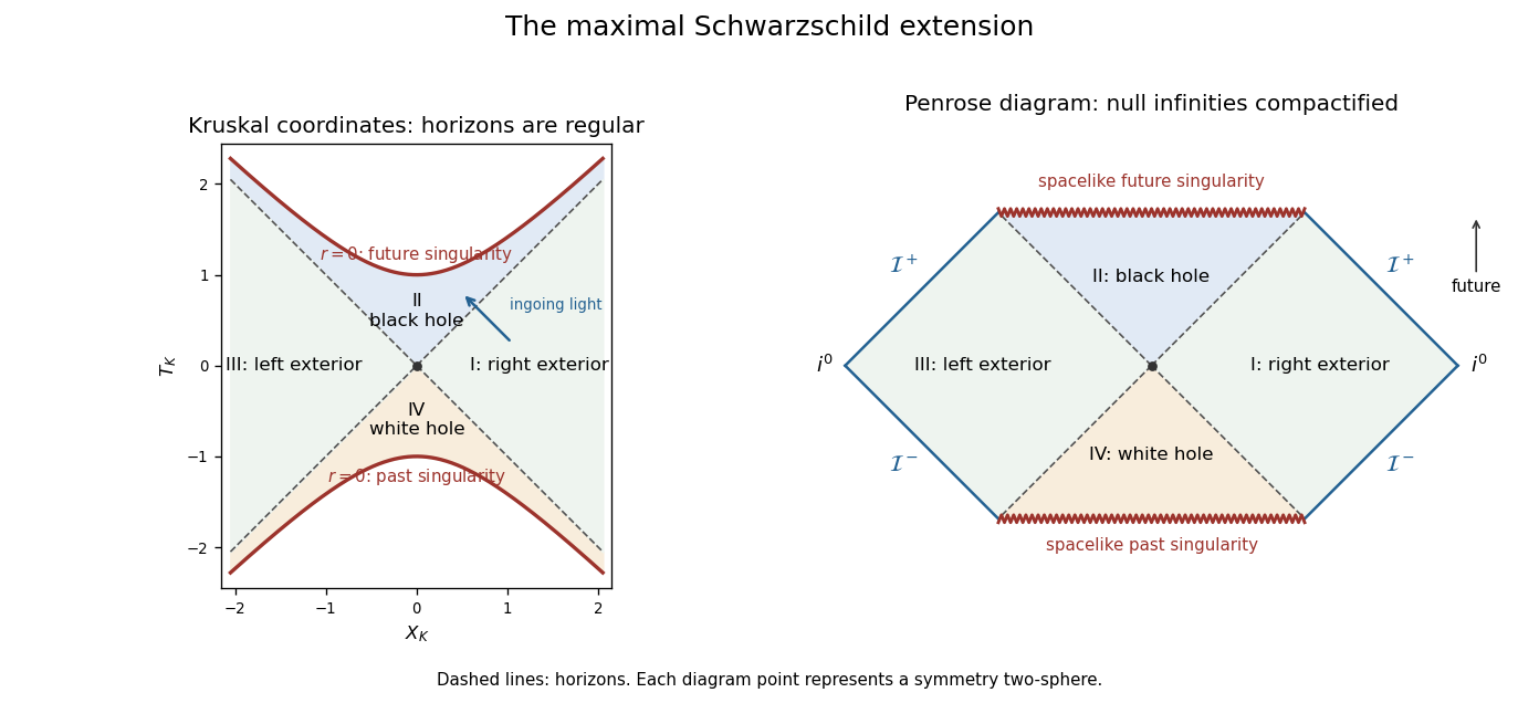
Kruskal and compactified diagrams of the maximal Schwarzschild extension, showing both exteriors, horizons and spacelike singularities
. Details. 
The time-symmetric spatial slice has a bridge between the exteriors, but it is not a traversable passage. Future-directed causal curves have nondecreasing and . Moving from the right exterior to the left would require to decrease from positive to negative; the reverse passage would require to decrease. Both are impossible. This proves the non-traversability of the Schwarzschild bridge. The complete eternal vacuum extension has two exteriors, a black hole and a white hole; it has no causal route between its exteriors. A black hole made by stellar collapse is a different global spacetime: its matter-filled past replaces the white hole region, and it normally has only one exterior. The vacuum extension constructed here should not be mistaken for the collapse history of a single star.
With electric charge, spherical electrovacuum instead gives the Reissner-Nordstrom metric, in an electromagnetic normalization absorbing the charge conversion constants:For , there are two simple horizons. Outside the metric is static; between and , and is timelike. Inside , again, so is spacelike and the singularity is timelike. The outer horizon is the event horizon; the inner horizon is a Cauchy horizon. The same logarithmic tortoise-coordinate and exponential-null-coordinate method crosses each simple horizon locally, but one exponential scale does not regularize both simultaneously: their surface gravities have different magnitudes,Continuing the exact metric through successive inner horizons produces repeated blocks with further exteriors, and evolution beyond a Cauchy horizon is not uniquely fixed by data on the original Cauchy hypersurface. The timelike singularity can be avoided by some trajectories in this ideal extension, unlike the unavoidable spacelike singularity of the future Schwarzschild spacetime interior. However, the enormous inner-horizon blueshift makes this exact continuation unstable: perturbations can cause mass inflation. This is an important qualification on the global structure of a charged spherical black hole.
At the two horizons coalesce, and surface gravity is zero. The horizon is a degenerate Killing horizon, the tortoise-coordinate divergence becomes a pole and the ordinary nondegenerate Kruskal spacetime construction must be replaced. The exterior develops an infinitely long spatial throat and the formal Hawking temperature vanishes. For , no real zero of remains: the electrovacuum solution has a naked singularity, not a black hole. Consequently arbitrarily allowing charge changes the causal structure, not just the horizon radius.
Past exam of the mathematics course of the University of Cambridge 2005 iii Paper 61 4 Solution Created 2026-10-03 Updated 2026-10-20
Use natural units, assume negligible neutrino chemical potentials, and approximate neutrino decoupling as occurring before electron-positron annihilation in cosmology. At high temperature, weak interactions maintain a common temperature for neutrinos, antineutrinos, electrons, Positrons and photons. Since , the reaction rate eventually loses against expansion. Decoupled relativistic neutrinos then free stream; their momenta redshift as , so their distribution retains a temperature parameter satisfying .
The still-coupled electromagnetic bath receives the entropy of annihilating electrons and Positrons. Its effective number of relativistic entropy degrees of freedom is initiallywhere the two photon polarizations count as bosonic states and the four electron-positron spin states have the fermion entropy weight . After the pairs disappear, . Cosmological entropy conservation in this coupled bath gives . The three already decoupled neutrino species are excluded from this bath's entropy count. At decoupling , henceSubsequent expansion preserves this ratio in the idealized history. Residual interactions during annihilation give small corrections to the instantaneous-decoupling approximation. If a relic species later becomes massive, here remains the redshifting momentum-distribution parameter; it need not be its nonrelativistic kinetic temperature.
A single ordinary neutrino species includes one populated neutrino helicity and one antineutrino helicity. For negligible chemical potential, integration of the Fermi-Dirac distribution givesTherefore the number density of a relativistic neutrino relative to photons, with the antiparticle included, isThe factor is the fermionic number-density weight, distinct from the energy and entropy weight . This relation continues to hold after this species becomes nonrelativistic if its comoving particle number is conserved.
Under the proposed matter-dominated, spatially flat model, the Friedmann equation requires the present relic-neutrino energy density to be approximately the critical density. Using the unreduced Planck mass givesThus the critical-density mass of a thermal relic neutrino isTaking the paper's rounded values, , and , givesFor , this is of order -- with these approximate constants. More precise constants change the coefficient, not the requested mass scale. This mass is much larger than the present momentum scale , validating the nonrelativistic energy density approximation. The result assumes that one thermal relic species dominates the matter density; it is conditional on that model rather than a measurement of a neutrino mass.
Past exam of the mathematics course of the University of Cambridge 2005 iii Paper 61 3 Solution Created 2026-10-03 Updated 2026-10-14
Use natural units and the unreduced Planck mass ; it is times the reduced Planck mass. A homogeneous canonical inflaton has and . Vacuum domination by a scalar field requires , with other matter and the curvature term negligible in the Friedmann equation. The equation-of-state parameter is then near , and the Friedmann acceleration equation gives accelerating expansion.
For sustained slow-roll inflation, Hubble friction must dominate the inflaton acceleration: , with the scalar potential changing only slightly in one Hubble time. In terms of the potential slow-roll parameter and second potential slow-roll parameter, this requiresFor the quartic scalar potential,Thus supplies a broad slow-roll range when . At an initial density of order the Planck density, potential domination givesso both potential slow-roll parameters are small for small . Small initial kinetic energy is a separate condition; the height of the scalar potential alone does not enforce it. These classical equations describe the post-Planck evolution under the model assumptions, rather than resolving quantum gravity at the initial endpoint.
Take ; the negative branch follows by the symmetry . Dropping kinetic energy from the Friedmann equation and acceleration from the inflaton equation of motion givesWriting , the quartic-potential slow-roll solution isIndeed, , and integrating gives . These expressions apply during slow-roll inflation; their formal late-time saturation must not be used beyond the end of that approximation.
The exact end of accelerating expansion is , equivalently for the scalar-dominated flat model. The quartic-inflation endpoint estimate uses the leading potential condition , givingThe numerical coefficient is an endpoint estimate: the slow-roll approximation breaks down there. Imposing estimates when slow roll loses accuracy and gives a different order-one coefficient, not a different exact acceleration condition.
The slow-roll e-fold count isThe quartic-inflation expansion from Planck density combines this initial estimate with the conventional endpoint to giveFor small the dominant term is enormous; the order-one endpoint uncertainty does not affect that conclusion.
To estimate the reheating temperature, assume prompt, efficient reheating converts the end-of-inflation energy into a thermal radiation bath. With the same endpoint convention, , and equating this to the radiation energy density givesThe quartic-inflation prompt-reheating estimate fixes the scaling; the endpoint kinetic energy changes the coefficient by order one. Without an inflaton coupling and its thermalization history, alone cannot specify the actual reheating temperature.
Finally, during cosmic inflation the comoving Hubble radius decreases:An initially causally connected patch is enlarged enough that the present observable region can lie within it. Its portions may subsequently be far outside one another's Hubble radii while retaining their common earlier thermal history. This solves the horizon problem if the number of e-folds is sufficiently large, conventionally of order sixty for the relevant thermal history; can readily exceed that. The necessary count depends on reheating and later expansion. The causal mechanism and the conversion back to a hot universe are discussed in David Tong's account of inflation.
There are unlisted articles, also show them or only show them.