
Past exam of the mathematics course of the University of Cambridge 2005 iii Paper 61 2 Solution Created 2026-10-03 Updated 2026-10-14
Use natural units and the unreduced Planck mass . Neutrino decoupling occurs when the weak interaction rate falls below the Hubble parameter. The weak-decoupling temperature estimate equates the given rate with the radiation-era expansion rate:Here counts the effective number of relativistic energy degrees of freedom, and the Fermi constant is . The omitted reaction-rate coefficients make this an order-of-magnitude estimate: decoupling occurs at a temperature of order one MeV.
The charge-conserving channel is , together with . The positron sign in the printed neutron-capture channel violates electric charge conservation. Chemical equilibrium requires . Negligible lepton chemical potentials therefore give . Since neutrons and protons are nonrelativistic particles, their Maxwell-Boltzmann distribution givesBoth nucleons have two spin states, and their masses agree closely in the prefactor. Thus neutron-proton chemical equilibrium impliesThe heavier neutron is suppressed by a Boltzmann factor.
For the deuterium equilibrium abundance, retain the paper's convention ; the positive nuclear binding energy is . Chemical equilibrium of gives because the equilibrium photon chemical potential vanishes. Using the nonrelativistic Maxwell--Boltzmann number density for each species and dividing givesHere and . With the baryon-to-photon ratio , the photon number density , and , , this becomesIn this convention counts nuclei, so its contribution to the fraction of baryons in deuterium is .
The deuterium bottleneck explains why helium-4 formation waits until is far below . At higher temperature, there are vastly more photons than baryons; even the dilute energetic tail can destroy newly formed deuterium. A crude estimate balances against one, giving for of order . The power-law factors in the deuterium equilibrium abundance and the nuclear reaction rates refine this estimate. Once stable deuterium accumulates, further reactions can efficiently place nearly all surviving neutrons into helium-4.
Write at the onset of nuclear burning. Each helium-4 nucleus requires two neutrons and contains four baryons. Neutron-limited helium synthesis therefore gives the primordial helium mass fractionFor a realistic rough cosmological weak freeze-out estimate, is about and free-neutron decay after freeze-out reduces it to about , giving roughly one quarter of the baryonic mass in helium-4. The survival relation that conserves baryon number is ; the corresponding is .
The rough neutrino decoupling rate by itself does not determine that one-quarter value. Substituting literally into would give and before neutron decay. Neutron-proton chemical equilibrium persists to a lower temperature, approximately -- once the actual conversion rates are included. The rate scaling fixes the MeV scale; accurate abundances need the conversion coefficients and the delay through the deuterium bottleneck. This sequence is described in David Tong's discussion of nucleosynthesis.
Increasing reduces the equilibrium neutron-to-proton ratio, so the primordial helium abundance decreases. Holding the freeze-out temperature and the decay survival factor fixed, the primordial helium response to the neutron-proton mass difference isFor and -- this is about --, a reduction of roughly fifteen percent. A larger also changes neutron decay and detailed weak rates; their quantitative effects require more microscopic information. The sign from the Boltzmann factor is already clear.
Past exam of the mathematics course of the University of Cambridge 2005 iii Paper 61 1 Solution Created 2026-10-03 Updated 2026-10-14
Use natural units with , write , and measure cosmic time from the Big Bang. The cosmological continuity equation follows by differentiating the Friedmann equation and using the Friedmann acceleration equation; for pressureless matter it gives , hence when the present scale factor is . The present critical density and cosmological density parameter giveConsequently, with , the Friedmann equation becomes .
Introduce conformal time through . A prime denotes a derivative with respect to , so andSet , with at the Big Bang. On the expanding branch the substitution satisfies this equation. Integrating , with , gives the closed matter-dominated Friedmann solution:The parametrization continues smoothly through the maximum scale factor, reached at , onto the contracting branch. Its curve in the plane is a rescaled cycloid.
For a presently expanding universe, selects . The normalization givesSubstitution yields the age of a closed dust universe:The first later zero of the scale factor occurs at , so the lifetime of a closed dust universe gives the Big Crunch timeThis is the total lifetime measured from the Big Bang; the remaining cosmic time is . As a check, the limit gives , while the Big Crunch recedes to infinite time, as expected for a flat matter-dominated universe with zero cosmological constant.
Past exam of the mathematics course of the University of Cambridge 2005 iii Paper 60 4 Solution Created 2026-10-03 Updated 2026-10-14
The physical spherical coordinates cover , , , and with periodic identification. The center and the polar axes are the usual coordinate singularities, rather than physical curvature singularities; a regular polar chart restricts and . For the null coordinates,Thus the physical metric tensor isThe conformal transformation followed by , gives , , andConsequently . Finally , converts to , yieldingThe ranges must retain their joint constraints:Equivalently, and , with . The angles retain their original ranges and identifications. Extending to negative values would double-count the radial polar geometry. The conformal factor isThe unphysical metric tensor extends onto the Einstein static universe, while physical Minkowski spacetime occupies the triangular region in its radial Penrose diagram. The edge is the regular center and belongs to the physical region away from its endpoints.
The conformal boundary consists of the following infinities. Future null infinity has , hence with , and corresponds to finite with . Past null infinity has , hence , and corresponds to finite with . Future timelike infinity is , past timelike infinity is , and spacelike infinity is . Although angles label points on null infinity, their two-spheres collapse at these three endpoint locations in the compactified picture.
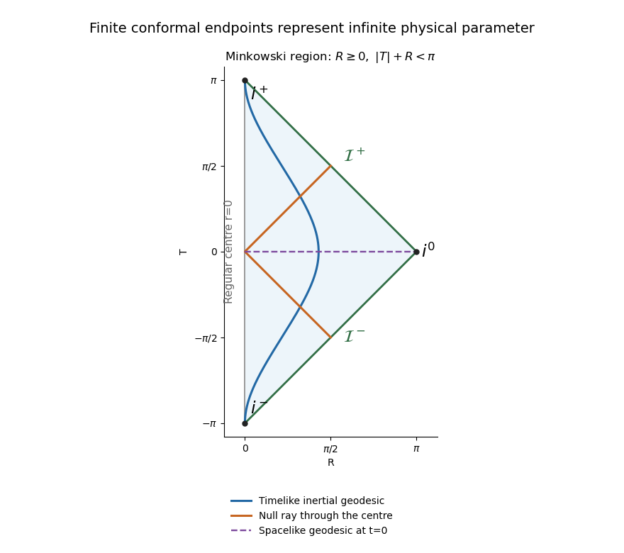
The radial Minkowski conformal diagram and the endpoints of timelike, null and spacelike geodesics
. Details. For the geodesic endpoints in Minkowski conformal compactification, one can check the limits directly. A timelike inertial trajectory is with . At both and tend to , so and the trajectory ends at future timelike infinity. At both tend to , giving past timelike infinity. This includes a stationary inertial worldline with bounded .
For a null inertial trajectory, . As , , so has a finite limit while ; its future endpoint lies on future null infinity. As , , giving a finite limiting and , hence a past endpoint on past null infinity. Radial null geodesic paths have constant. A ray passing through the center changes its angular direction; in the angle-suppressed radial diagram it reflects at rather than terminating there.
A spacelike geodesic is also a straight line, now parametrized so that . At either end, asymptotically, , , and the endpoint is spacelike infinity. A radial spacelike line at has two opposite-angle halves which project onto the same horizontal interval in the diagram.
The conformal compactification endpoints occur at finite but at infinite physical proper time or affine parameter; Minkowski spacetime is geodesically complete. The conformal preservation of null geodesic paths does not preserve an affine parameter: if is physically affine, an unphysical affine parameter satisfies up to a constant. Along a complete null ray this can have a finite integral at infinity. Timelike and spacelike physical geodesic paths are not generally geodesics of the rescaled metric tensor, so their drawn curves must not be interpreted as freely falling unphysical observers.
Finally, every physical event can send an outgoing null ray to future null infinity, so is all of Minkowski spacetime. Its black-hole region and intrinsic event horizon are empty. The null edges in the diagram are infinity, not horizons concealing part of the physical manifold. Complete inertial observers likewise have no observer event horizon. Accelerated observers restricted to a Rindler wedge can have a Rindler horizon, but that is observer-dependent and does not contradict the horizon-free Minkowski spacetime. The conformal diagram compactifies infinity; it does not introduce a physical horizon.
Past exam of the mathematics course of the University of Cambridge 2005 iii Paper 60 3 Solution Created 2026-10-03 Updated 2026-10-14
For the static nonrotating source, use spherical symmetry and the static scalar perturbation of Minkowski spacetime, with isotropic radius :To first order, the Einstein tensor in the declared convention hasThese are also the static scalar perturbation of Minkowski spacetime equations in the original information sheet. The source has and zero spatial stress. With the sign established in Question 2,The distributional identity and asymptotic flatness give . For , the spatial field equation has trace and therefore . Its decaying spherical solution is , so . This determines both potentials; the spatial correction cannot be inferred from the Newtonian gravitational potential alone.
Now use the isotropic-to-areal weak-field radius change. The angular coefficient defines , hence to first order. Thus to the same accuracy, and replacing by inside a perturbation changes only second-order terms. With the Schwarzschild radius , the linearized Schwarzschild metric isThis is an exterior weak-field approximation: . The point source is used distributionally to fix the mass, not to claim a regular or weak field at the origin.
For a null geodesic choose its orbital plane as , using rotational symmetry, and let a dot denote an affine parameter derivative. For a Killing vector and an affinely parametrized geodesic tangent , the geodesic conserved quantity from a Killing vector follows directly fromApplying this to the time-translation and axial Killing vectors, with the spatial sign absorbed into the definition of , givesIf the tangent is normalized as the photon's four-momentum, is its energy measured at infinity and its signed angular momentum about the selected axis. Rescaling an arbitrary affine parameter rescales both; the ratio is the invariant impact parameter. Future-directed orbits have . Assume to use as the orbit parameter; gives radial rays, not a finite-radius circular orbit.
The null vector constraint givesExpand consistently to first order in the weak-field approximation correction: and . Also . Therefore the first-order orbital equation isThe cubic term is the first correction relative to the flat inverse-radius term; the equation is not a controlled exact equation for large .
A constant solution of a first integral is not by itself sufficient to establish a circular geodesic. For a circular trajectory, the radial Euler-Lagrange equation also requires , where now is the metric's time coefficient. Combining this with the null vector constraint gives , or . Equivalently, the formal potential must have a stationary point. Apart from the infinite-radius endpoint , its only stationary point is , with . Thus the formal circular solution requiresThe reduced radial equation is , with prime denoting . It follows by differentiating the first integral on moving segments and agrees with the regular Euler-Lagrange equation at turning points. Perturbing givesThere is an exponentially growing linear instability mode; equivalently . The formal circular orbit is unstable.
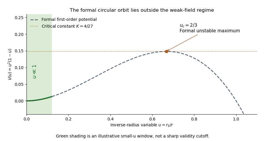


The weak-field photon-orbit validity limitation is essential: is not small. There is therefore no finite-radius circular photon orbit established within the controlled weak-field region. The formal extrapolation happens to reproduce the radius and impact parameter of the exact Schwarzschild photon sphere, but that physical result needs the exact geometry. The calculation also cannot establish a Schwarzschild event horizon from a first-order expansion at .
Past exam of the mathematics course of the University of Cambridge 2005 iii Paper 60 2 Solution Created 2026-10-03 Updated 2026-10-14
General relativity models spacetime by a smooth four-dimensional Lorentzian manifold whose metric tensor governs clock readings, causal cones and free-particle motion. The Einstein equivalence principle motivates local special relativity and universal geodesic free fall for test bodies; it does not by itself select a unique gravitational field equation. We assume a Levi-Civita connection, a metric tensor as the gravitational field with no additional dynamical gravitational variables, and matter with a covariantly conserved stress-energy tensor. Units have .
The existence of local inertial frames is a local statement. At any regular event choose an orthonormal frame and Riemann normal coordinates, so that and at the event, with metric signature . Metric compatibility then gives there. The geodesic equation at that point is the special-relativistic inertial equation. Along a timelike geodesic, a parallel-transported orthonormal frame gives Fermi normal coordinates, eliminating the connection along the central worldline. These constructions do not in general eliminate second derivatives of the metric tensor in a neighborhood. The Riemann curvature tensor is built from the derivatives of the connection coefficients as well as their quadratic terms; nonzero Riemann curvature tensor components can remain when all connection coefficients vanish at a chosen point. Conversely, Polar coordinates in Minkowski spacetime can have nonzero connection coefficients but zero Riemann curvature tensor. Connection coefficients alone are therefore not an invariant measure of gravity.
For the tensorial content, consider a two-parameter family of geodesics parametrized by an affine parameter, with tangent and connecting field . Their coordinate construction gives , and torsion-freeness gives . Since , commuting derivatives in the convention of Question 1 yields geodesic deviation:The left side is covariant relative acceleration, rather than the second coordinate derivative of an arbitrary separation. In an orthonormal frame in free fall with , its spatial components are . This is a measurable tidal force, and a coordinate transformation cannot make a nonzero Riemann curvature tensor disappear. It is the distinction between gravity at one event and the behavior of an extended freely falling laboratory.
In a static Newtonian limit, and , so the test-body acceleration is . The curvature-sign convention in Killing derivative identities gives . Hence relative acceleration is the negative Hessian of the gravitational potential. For the Newtonian potential of a point mass , the Hessian has radial eigenvalue and two tangential eigenvalues : radial separations stretch and tangential ones compress. Outside the source the Ricci tensor can vanish while the Riemann curvature tensor remains nonzero. Its vacuum tidal part is encoded by the Weyl tensor; vacuum does not mean flatness. Gravitational waves likewise carry Riemann curvature tensor disturbances without a local material source.
To obtain the field equations, make the additional dynamical assumptions explicit: locality and diffeomorphism invariance of general relativity; a symmetric metric tensor field equation using at most second derivatives of the metric tensor; a geometrical left-hand side linear in the Riemann curvature tensor with constant coefficients; and compatibility with local matter conservation. These restrictions exclude higher-curvature or extra-field alternatives. Under them the available rank-two curvature contractions give the ansatzThe contracted Bianchi identity and metric compatibility giveFor this to vanish identically for arbitrary metric tensors, . Assuming and absorbing its normalization into the coupling givesThe permitted constant term is the cosmological constant. Its value is not fixed by the equivalence principle. Conservation of follows for generally covariant matter on its equations of motion: varying the matter action under a compactly supported infinitesimal diffeomorphism, then integrating its term by parts, gives . The divergence-free Einstein tensor is consistent with this identity.
The coupling sign must be fixed in the actual curvature-sign convention in Killing derivative identities, with . For the static weak-field approximation, . Set for the local asymptotically flat Newtonian comparison. In four dimensions the trace equation gives , so for slowly moving matter. Matching forces . Thus, with this convention,Under the opposite curvature-sign convention in Killing derivative identities the coupling sign reverses, as in Einstein-equation coupling under reversed curvature. This sign statement is compatible with the supplied linearized handout. Local inertial frames remove the connection at an event; tidal Riemann curvature tensor effects remain tensorial, and the field equations require dynamical assumptions beyond the equivalence principle.
Past exam of the mathematics course of the University of Cambridge 2005 iii Paper 60 1 Solution Created 2026-10-03 Updated 2026-10-14
For a scalar, the Lie derivative of a function is its directional derivative:The Lie derivative of a vector field is their Lie bracket of vector fields:For a torsion-free connection,The last term vanishes because the connection coefficients are symmetric in . This proves .
For the metric tensor statements use the Levi-Civita connection, which also has metric compatibility. The tensor derivation property of the Lie derivative of a tensor field givesExpanding the first term using and using the vector identity cancels the derivatives of and . What remains isSince are arbitrary, the Killing equation isMetric compatibility is needed here, even though symmetry alone sufficed for the vector identity. In general the Lie derivative of a metric with nonmetricity contains a term . For example, with the metric tensor , zero connection coefficients and , the Lie derivative of a tensor field is , whereas . The usual metric connection interpretation of the question supplies the required compatibility.
For the Riemann curvature tensor calculation, keep the original PDF's convention. With and , it meansThus the commutator on a covector has the opposite sign. Write . Taking a covariant derivative of the Killing equation makes antisymmetric in its first two indices, while the Ricci identity givesCombining this with the first-two-index antisymmetry gives the three relationsAdd the first and third and subtract the second. Pair symmetry and the first Bianchi identity imply . ConsequentlyThis is the second covariant derivative of a Killing vector in the paper's convention; its sign is tied to the declared curvature-sign convention in Killing derivative identities, not to raising a particular index.
Set . Along any smooth curve with tangent vector , the chain rule and the just-proved identity give the Killing transport equationsChoose a parallel-propagated orthonormal frame along the curve. These become a homogeneous linear system of ordinary differential equations for the components of . Uniqueness of its initial value problem implies that zero initial data remain zero. Any point in the same connected component as can be joined to by a piecewise smooth curve. Therefore zero value and zero first derivative at force the Killing field and its derivative to vanish throughout that component, with no completeness assumption. On a manifold with one connected component this is the requested global result. Connectedness cannot be dropped: on two disjoint flat spacetimes, take the zero field on one and a nonzero translation on the other.
On a pseudo-Riemannian manifold of dimension with one connected component, the map is therefore injective. There are independent components of the value and of its antisymmetric derivative. The dimension bound for Killing vector fields isIt is attained in flat space by with constant antisymmetric , giving translations and infinitesimal rotations or Lorentz transformations. The four-dimensional maximum is 10. For a disconnected manifold the bound applies componentwise; there is no uniform global bound depending only on if the number of components is unrestricted.
Past exam of the mathematics course of the University of Cambridge 2005 iii Paper 6 4 Solution Created 2026-10-03 Updated 2026-10-14
We construct the finite evaluation representation explicitly by Lagrange interpolation. This supplies all the polynomial facts needed for the bound.
Define the Chebyshev polynomial by andInduction shows that has degree ; the cosine addition identity also proves . Therefore , and follows from the recurrence. The case is immediate, since both and are constant.
For , choose the descending extremal nodesso . Define the fundamental interpolation polynomialsThey satisfy . Consequentlyfor every polynomial of degree at most : the difference has degree at most and vanishes at the distinct nodes, so it is zero. The root count used here follows by successively factoring from a polynomial having such a root; a nonzero degree- polynomial cannot have more than distinct roots. Thus the interpolation identity has been proved.
If , every numerator factor in is positive, while exactly denominator factors are negative. Hence . Applying interpolation to itself givesPutting in the interpolation formula yieldsFor , apply the proved positive-side inequality to at , and use the parity identity. The result isThis is sharp, with equality for or its scalar multiples.
In functional terms, the evaluation map on the normed polynomial space has : the inequality gives the upper bound and attains it. For , its normalized version has the exact representationThus Chebyshev interpolation represents external evaluation using nodes. The necessary finite representation and its norm are derived directly, so no convex-hull theorem is being invoked without proof.
Past exam of the mathematics course of the University of Cambridge 2005 iii Paper 6 3 Solution Created 2026-10-03 Updated 2026-10-14
Use a nonzero complex unital Banach algebra with submultiplicative norm, and write its unit as . The complex scalar field is the usual convention in this spectral statement; for a real algebra one uses its complexification. We derive the needed analytic facts from norm-convergent series and scalar complex analysis.
If , completeness makes the Neumann series converge. Multiplying its finite partial sums by gives , which tends to . Hence its sum is the inverse of . If is invertible, then is invertible whenever . This proves that the invertible elements form an open set and that inversion is locally norm-continuous.
Define the Banach algebra spectrum and the resolvent of an element byFor , the Neumann series givesThus is bounded by and is closed, because invertibility is open. Also in norm at infinity; for example its norm is at most , since in a nonzero submultiplicative unital algebra. The standard normalization is not needed.
For points where the Banach algebra resolvent exists , multiply out the inverses to get the resolvent identityFor outside the Banach algebra spectrum, put . Locally,This series and its differentiated series converge uniformly on every smaller disk. It therefore proves is a Banach-space-valued holomorphic function, establishing complex differentiability in the Banach-space norm and gives , without assuming a Banach-algebra-valued analytic theorem. In particular every continuous complex linear functional makes a scalar holomorphic function.
The Banach algebra spectrum is nonempty. Otherwise would be defined and analytic everywhere. Its local norm continuity and decay at infinity make it globally bounded. For every continuous linear functional , the scalar entire function is bounded and tends to zero at infinity, so it is identically zero: the scalar Cauchy estimate for its derivative on circles of radius is , which tends to zero, and the limiting value then fixes its constant as zero. Such functionals separate points by the Hahn-Banach theorem. Explicitly a bounded real functional can be extended from the real span of any nonzero element using its norm, and complexifying it by gives a bounded complex linear functional nonzero on that element. Therefore itself would be zero, contradicting . We have proved the Banach algebra spectrum is a nonempty compact subset of the complex plane.
We next establish the spectral radius formula. The power norms are submultiplicative. If some , their root norms are eventually zero. Otherwise, for any fixed , write with to obtainTaking roots gives . Taking the infimum in , and using that every root norm is at least that infimum, proves existence ofFor , the root test makes converge, even when . The same telescoping multiplication proves it is a two-sided inverse. HenceFor the reverse bound fix . If , integrate the uniformly convergent exterior series term by term on , obtainingThe same integral equals the one on : applying an arbitrary continuous linear functional reduces contour deformation through the Banach algebra spectrum-free annulus to the scalar Cauchy theorem, and separation of points restores equality in . This proves the resolvent Cauchy coefficient formula rather than assuming vector-valued analytic calculus. Using the norm bound for the allowed vector integral givesTaking th roots yields , and letting finishes the proof:
For the first example take the commutative algebra of dual numbers with norm . Completeness follows from finite dimension, and the product estimate makes the norm submultiplicative. For , but , so . Directly, has inverse for , and its Banach algebra spectrum is . For the second example take with its absolute-value norm and . Its Banach algebra spectrum is , giving .
Past exam of the mathematics course of the University of Cambridge 2005 iii Paper 59 4 Solution Created 2026-10-03 Updated 2026-10-14
Let . An arbitrary deterministic strategy, including auxiliary systems, intermediate measurements, adaptive actions and discarded records, is a quantum channel from the two input qubits to the three returned qubits. Its output is . The three local tests commute, and their joint all-pass projector is . Thusis exactly the probability of at least one failed test. No independence of the three returned qubits is assumed.
We prove a uniform positive obstruction using trace distance, . Two normalized pure kets obeyIndeed their projector difference is supported on their two-dimensional span, has trace zero, and has eigenvalues .
Two further estimates will cover even mixed outputs. First, trace distance contracts under a quantum channel. To see this directly, the positive spectral projector of the trace-zero difference gives . The adjoint of a channel is positive and unital, so it takes any output effect into an input effect. Maximizing over this subset cannot exceed the input maximum, proving contraction.
Second, for a mixed state and a pure target , the trace-norm triangle inequality and weighted Cauchy-Schwarz inequality give the pure-target upper bound on trace distance:In particular .
Now take and . The two-copy input distance is , whereas the ideal three-copy distance is . Writing , contraction and the triangle inequality yieldLet . Then , and squaring givesThis is the copy-number trace-distance obstruction. It applies to every Bob strategy, irrespective of its internal complexity. If Alice chooses these two possible inputs with equal probabilities, the left side is her unconditional failure probability. For every device, at least one of the two inputs also has failure probability at least , establishing the worst-case guarantee.
The same positive bound holds if Alice chooses a uniformly random pure-qubit state. Apply the preceding inequality to and for every single-qubit unitary , since their overlap is unchanged. Average over normalized Haar measure. Both rotated kets have the same uniform distribution on the Bloch sphere, so each of the two average failures is the uniform-input average. Consequently that average is also at least . A constant satisfying the strict requested inequality in either this average or the worst-case interpretation isThe proven bound is , hence strictly greater than . This proof establishes a quantitative gap, rather than relying only on the impossibility of exact quantum cloning.
There is a necessary quantifier qualification because the PDF does not specify Alice's input distribution. A positive lower bound for every fixed state against every strategy would be false: a device hardwired to return never fails when the input is . The unknown-state assertion is therefore meaningful as a worst-case guarantee over possible inputs, or as an average for a specified hidden input ensemble. Both the equal-prior example and the uniform-input version have been proved here, with a constant independent of Bob's strategy.
Past exam of the mathematics course of the University of Cambridge 2005 iii Paper 59 3 Solution Created 2026-10-03 Updated 2026-10-14
Perfect identification on every trial is impossible, because the family contains a nonorthogonal pair. Any physical identification device induces a POVM whose effect corresponds to its declaration of label . Certainty of correct identification would require and for every .
Since , the first identity gives , while positivity and the second identity give . For example these conclusions follow by writing the zero expectations as squared norms of and . ThusPerfect identification would force the entire family to be orthogonal, contrary to the hypothesis. This argument permits ancillas, general measurements and disturbance of the input; it does not assume that the device must preserve the state.
Unambiguous identification with a nonzero success probability for every input is possible. Normalize the given kets and let be their Gram matrix. Their linear independence makes positive definite. Define reciprocal vectors within their span byThen , and hence also . Put . It is positive and has finite operator norm. Choosing , setAll these effects are positive, and , so they sum to the identity and define a POVM. The Born rule givesThus every label is correct whenever it occurs and every input has the strictly positive success probability . This is the reciprocal-state construction of unambiguous discrimination.
For an explicit success constant, collect the input kets into a matrix , so . Its polar factorization is with . The reciprocal columns are , and therefore . Its largest eigenvalue is , so one can take . Since the normalized Gram matrix has trace , this is at most .
To realize the device, use measurement operators and . The map preserves inner products because the effects sum to . Extend this linear isometry to a unitary on the input and an initially blank ancilla, then projectively measure the ancilla's orthogonal outcome labels. Its outcome probabilities are precisely those above. This gives a physical unambiguous quantum state discrimination device rather than only a formal set of effects.
Past exam of the mathematics course of the University of Cambridge 2005 iii Paper 59 2 Solution Created 2026-10-03 Updated 2026-10-14
The Schrödinger–Jaynes–Hughston–Jozsa–Wootters theorem classifies all finite quantum state ensembles of a density matrix. Write its nonzero spectral decomposition as , with and orthonormal eigenvectors. An ensemble with subnormalized vectors , , represents exactly whenHere is an column linear isometry. Zero-weight vectors may be included or discarded. Equivalently, any two ensembles represent the same density matrix if and only if, after padding the shorter list with zero vectors, their subnormalized vectors are related by a unitary matrix acting on the ensemble index. This is the isometry parametrization of a density-matrix ensemble.
For necessity, if lies in the kernel of , thenEvery therefore lies in the support of . Define . The ensemble identity givesso these columns are orthonormal and the displayed parametrization follows.
Conversely, start with any such isometry and define by the boxed equation. ThenThe weights are and sum to . Normalize every nonzero to obtain its pure state. This proves both directions and includes degenerate eigenvalues without any preferred choice of basis in their eigenspaces.
To prove the unitary-mixing version, pad two ensembles to a common length . Their matrices and have orthonormal columns in . Extend each column family to an orthonormal basis, obtaining square unitaries and . Then is unitary and , so the second ensemble vectors satisfy . Conversely this unitary mixing preserves , because . Independent phase choices for ensemble kets are absorbed in the row phases of these matrices.
The classification also has a measurement interpretation. Purify as . On the ancillary system define . The effects sum to , hence form a POVM. The conditional unnormalized system ket is , with probability . Thus every ensemble can be realized by measuring a purifying system; with a sufficiently enlarged ancilla the measurement can be projective. The density matrix specifies the common statistics without selecting one particular ensemble decomposition.
Past exam of the mathematics course of the University of Cambridge 2005 iii Paper 59 1 Solution Created 2026-10-03 Updated 2026-10-14
Apply the Schmidt decomposition to the bipartite pure state. Local unitary operators put it in the form , with after interchanging basis vectors. Both Schmidt coefficients are nonzero because the state is entangled. Put .
For this state, direct application of the Pauli operators givesFor example interchanges and , giving ; the crossed products take these two kets into their orthogonal complement.
Choose the CHSH axes for an entangled pure two-qubit state:Their associated Bloch vectors have unit length, so each is a valid two-outcome projective measurement with projectors or . The correlation combination isA local hidden-variable assignment with outcomes gives absolute value at most two: exactly one of and vanishes, while the other is . Averaging these assignments preserves that bound, which is the CHSH inequality.
Therefore . For the original state , conjugate Alice's observables by and Bob's by . These conjugations rotate their measurement axes and preserve all the displayed correlations. Thus every entangled pure two-qubit state has the requested violating axes. The maximally entangled case gives , while the unentangled limit merely saturates two.
There are unlisted articles, also show them or only show them.