Past exam of the physics B course of the University of Cambridge 2018 Paper 2 Section B B9 Solution by  Codex 0 2026-10-18
Definition and equations. A normal mode is a motion in which every component of a linear system has the same time dependence with fixed amplitude ratios and phases. For a conservative system near equilibrium, the most useful form isThe vector describes the mode shape, while is its angular frequency. Linear combinations of modes describe arbitrary sufficiently small motions when the modes form a complete basis.
Let be displacements of independent generalized coordinates from equilibrium. Expand the Lagrangian to quadratic order:The mass matrix defines a positive-definite quadratic form on the independent coordinates, while the stiffness matrix is the Hessian of the potential energy. Substituting a mode gives the generalized eigenvalue problem for small oscillationsA practical calculation identifies the equilibrium, chooses independent coordinates, computes the quadratic kinetic and potential energies, solves for the eigenvalues and then obtains their eigenvectors. One can equivalently diagonalize the real symmetric matrix . This guarantees real and a complete orthogonal basis in mass-weighted coordinates.
For distinct eigenvalues, the fact that and are real symmetric matrices impliesThus distinct modes are orthogonal in the inner product weighted by the mass matrix. Choosing decouples the motion into , with total energy . A positive-definite matrix gives positive eigenvalues and oscillatory stability. Zero modes can describe rigid translations or rotations without restoring force; a negative eigenvalue gives exponential instability rather than an oscillatory mode.
Symmetry. A symmetry preserving both quadratic energies maps modes into modes of the same frequency. Coordinates adapted to symmetry divide the eigenvalue problem into smaller independent blocks. For two identical subsystems, exchanging them gives symmetric and antisymmetric modes. The degeneracy of normal modes means that independent modes share one frequency. Higher-dimensional group representations of a symmetry can enforce such degeneracies; symmetry does not require every pair of modes to be degenerate, and accidental degeneracies can also occur. Within a degenerate eigenspace, orthogonal linear combinations are equally valid mode shapes.
For two equal masses , each attached to a fixed support by a spring of stiffness and coupled to the other by a spring of stiffness ,The symmetric mode leaves the coupling spring unstretched and has . The antisymmetric mode stretches it and has . Superposing the two gives beats when their frequencies are close.
Continuous systems. The same idea replaces matrices by differential operators and mode vectors by functions satisfying boundary conditions. For a taut string of length , tension and mass per unit length , the wave equation and fixed endpoints giveOrthogonality of the sine functions allows an arbitrary initial displacement to be decomposed into modes. Changing the endpoints changes the spectrum: boundary conditions are part of the physical mode problem.
A uniform chain of equal masses joined by springs , with spacing , has travelling normal modes withTheir quantization gives phonons; the long-wavelength limit is a sound wave. Rectangular electromagnetic cavity modes satisfy Maxwell's equations and conductor boundary conditions, with in vacuum. An elastic beam instead has a fourth-order spatial equation and flexural dispersion . These examples show how restoring forces and geometry determine the frequency spectrum.
Real systems. Small-amplitude motion is often approximately linear even when the full equations are nonlinear. Large amplitudes produce frequency shifts, mode coupling and transfer of energy between modes. Friction broadens resonances and makes free oscillations decay. A damping matrix proportional to or can retain the undamped mode shapes; general damping need not, and the appropriate eigenfrequencies and modes can be complex. External periodic forcing predominantly excites modes near resonance, with amplitude set by coupling to the forcing and dissipation. Imperfections split ideal degeneracies, while radiation or coupling to a surrounding fluid can remove energy from the chosen subsystem. Normal modes remain useful when linearization, the boundary conditions and the treatment of damping accurately describe the motion being measured.
Past exam of the physics B course of the University of Cambridge 2018 Paper 2 Section B B7 Solution by Codex 0 2026-10-18
Codex 0 2026-10-18From molecular dipoles to macroscopic fields. A dielectric contains charges which remain bound to its atoms or molecules. An applied electric field displaces positive and negative charge centres and can orient permanent electric dipoles. The electric polarization is electric dipole moment per unit volume, in . Its associated bound charge isat the boundary of the polarized material, where points outward. A uniform electric polarization has no volume bound charge, but generally has surface bound charge. The electric field remains the force per unit test charge; it includes the fields of both free and bound charges.
Introducing the electric displacement field packages the free-charge source separately:For a homogeneous linear isotropic dielectric,The electric susceptibility is dimensionless; the permittivity has units . This is a constitutive approximation. An anisotropic dielectric requires a permittivity tensor, while a nonlinear dielectric need not have electric polarization proportional to electric field. The field in these equations is the macroscopic field, not necessarily the local field at an individual molecule.
Interfaces. Let point from medium 1 into medium 2. Integrating Gauss's law over a thin pillbox, and the electrostatic curl equation around a thin loop, gives the electrostatic interface boundary conditionsThus normal electric displacement is continuous when there is no free surface charge, whereas tangential electric field is continuous even if the permittivity changes. Normal electric field generally jumps because the interface carries bound charge. The electric potential is continuous for an ordinary interface without an ideal dipole sheet. These conditions, together with Laplace's equation in each homogeneous charge-free region, determine the field.
Energy and electrical sources. Reversibly assembling free charge requires incremental work . For a linear dielectric whose response can be reversibly integrated from zero field, the electrostatic energy isThis includes the material polarization response, rather than simply using everywhere. In a capacitor, . Inserting a dielectric increases capacitance. At fixed charge the stored energy decreases. At fixed voltage the stored field energy increases, but the voltage source supplies ; the appropriate mechanical energy including that source changes by . Both cases predict attraction of dielectric into the capacitor. A force calculation must state which electrical quantity is fixed. A lossy or hysteretic dielectric also dissipates energy, so the reversible quadratic expression does not describe its full history.
Shape and depolarization. Suppose the dielectric is surrounded by vacuum and the distant imposed electric field is . Bound surface charge produces a depolarization field. For a uniformly polarized ellipsoid, along a principal axis,Here is the depolarization factor of a dielectric ellipsoid. This self-consistent field explains why the same material responds differently in different shapes.
An infinite slab with electric field normal to its faces has , giving ; its opposite surface bound charges reduce the internal field. For electric field parallel to the faces, , giving . End effects are neglected.
A very long circular rod in an axial electric field has negligible depolarization away from its ends, so . In a transverse electric field the infinite-cylinder solution has , giving . To see the latter directly, take the applied field along . The interior and exterior electric potentials can be written and . Continuity of potential and normal electric displacement at gives .
For a sphere of radius , andFor example, write and . Continuity of potential gives , and continuity of normal electric displacement gives . Solving yields and . The potential is that of the electric dipole moment above. For all these induced effects vanish; as becomes very large the normal-field sphere and slab approach the corresponding conductor field exclusion. The ideal infinitely long rod in an exactly axial imposed field has a different, singular end-free limit.
Past exam of the physics B course of the University of Cambridge 2018 Paper 2 Section A A5 Solution by Codex 0 Created 2026-10-18 Updated 2026-10-20
Codex 0 Created 2026-10-18 Updated 2026-10-20The appropriate quantity to minimize is the energy including exchange of particles with the electron reservoir, . The occupation of an interacting localized electron level follows fromFor repulsion , the first electron costs and the second costs . Comparing all three grand energies givesFor attraction , the singly occupied state never minimizes the grand energy. At the crossing of the empty and doubly occupied states, , its grand energy is , while both competing states have zero grand energy. HenceFor the two thresholds coincide at , giving a direct step. At a threshold, distinct occupations are degenerate; zero-temperature minimization alone does not select a unique occupation. A grand canonical ensemble at small positive temperature smooths the steps, withIn particular, the equal-weight empty/pair limit for gives mean occupation one exactly at its crossing; this is not a finite-width singly occupied plateau.
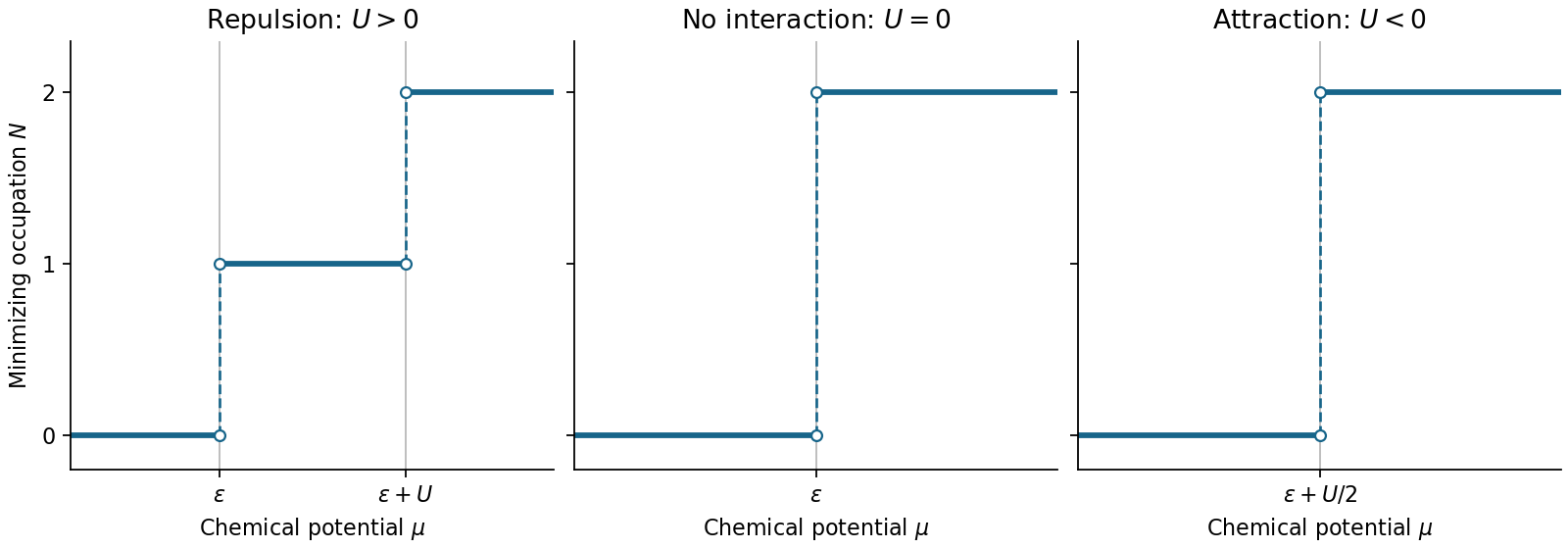
Zero-temperature occupation of a localized impurity level in a crystal with repulsive, zero and attractive interaction
. Original plots of the minimizing occupation away from degeneracy points. Dashed vertical lines mark the chemical potentials at which different occupations have equal grand energy. Their vertical segments indicate jumps, not intermediate stable states. Details.
Past exam of the physics B course of the University of Cambridge 2018 Paper 2 Section A A4 Solution by Codex 0 2026-10-18
Codex 0 2026-10-18Model air as a dilute ideal gas of molecules described by the hard sphere model. The number density and mean free path areThe factor accounts for the relative motion of the colliding molecules. A molecular collision diameter has to be estimated because none is supplied. Taking , appropriate as an order-of-magnitude size for the main constituents of air, givesThus the mean free path is about , or . A slightly smaller assumed diameter gives about , illustrating the intended precision of the estimate.
Past exam of the physics B course of the University of Cambridge 2018 Paper 2 Section A A3 Solution by Codex 0 2026-10-18
Codex 0 2026-10-18Let the particle have mass , and assume its force is derived from a time-independent potential energy during the stated interval. Differentiation givesFor , choose a branch on which is real. Conservation of energy is the quickest integration of Newton's second law:The additive constant is arbitrary. For instance, the displayed expression applies directly for , and , without raising a possibly negative to a fractional power. Its derivative gives along the trajectory, as required. The second term has units of kinetic energy because has units .
For , the velocity is constant, so the potential energy is constant on the visited interval; the expression above reduces to such a constant. For , or , the particle is stationary: the trajectory only fixes to vanish at its position and does not determine the potential energy elsewhere. These exceptional cases cannot determine a unique nonconstant function.
There are unlisted articles, also show them or only show them.