Past exam of the physics course of the year 1 of the natural sciences course of the University of Cambridge 2021 Section B 9 b Solution by  Codex 0 2026-10-18
Keep the paper's as magnitudes for the two convex faces. With the standard signed-curvature convention measured to the right, the first surface has signed radius and the second . This explains why the requested formula contains a sum of the two reciprocal magnitudes.
Let the axial lens thickness be , and let be the distance from the first vertex to the intermediate focus that its refracted rays would reach without the second surface. The first refraction at a spherical surface givesAt the second face those rays are still converging toward that intermediate focus, so its object distance is negative, , with . Applying the signed spherical-surface equation again givesIn the thin lens limit, . Adding cancels the intermediate-focus terms:The focal length is the image distance for parallel incident light rays, , hence the lensmaker's equation isThe same surrounding refractive index is assumed on both sides. For this biconvex thin lens has positive focal length. With signed radii , , the equivalent familiar expression is .
Past exam of the physics course of the year 1 of the natural sciences course of the University of Cambridge 2021 Section B 9 a Solution by Codex 0 2026-10-18
Codex 0 2026-10-18Use the original diagram's positive distances: from the object to the vertex, from the vertex to the image, and from the vertex toward the centre of curvature on the outgoing side. Let a paraxial light ray strike at height . Its incoming inclination is above the optical axis, its outgoing inclination is below it, and the inward surface normal is inclined by below it. Thus the incidence and refraction angles relative to that normal are respectively and .
The local tangent-plane form of Snell's law, using the small-angle approximation, givesSubstitute the three height-to-distance ratios and cancel :This refraction at a spherical surface result keeps only first-order ray angles. The surface sag shifts the height's axial reference only at higher order. Distances for other object, image or curvature orientations must be signed consistently; the displayed positive-distance form follows the particular orientation in the paper.
Past exam of the physics course of the year 1 of the natural sciences course of the University of Cambridge 2021 Section B 8 g Solution by Codex 0 2026-10-18
Codex 0 2026-10-18For overdamping, . Put . Both characteristic roots are negative real numbers. Replacing trigonometric functions by hyperbolic functions gives the exact trajectoryIt starts from with tangent , bends anticlockwise toward the origin, and approaches it without repeated revolutions. The right panel gives a representative choice ; the paper does not specify one particular value of in this regime.
One can make the qualitative shape precise. In radial and tangential directions relative to the initial radius, the angle turned from the starting direction obeysFor , both coordinates stay positive, and the approach is along the fixed ray with . The initial velocity is tangential, so an immediately straight radial return would be incorrect. The absence of oscillatory characteristic roots prevents repeated revolutions. This is a non-spiralling overdamped central oscillator trajectory.
Past exam of the physics course of the year 1 of the natural sciences course of the University of Cambridge 2021 Section B 8 f Solution by Codex 0 2026-10-18
Codex 0 2026-10-18The parameters giveThe coordinate expressions for the initially circular damped planar oscillator areThe damped oscillation period gives almost four anticlockwise turns in four seconds. The radius envelope falls by . Substitution into the exact coordinates givesThe left panel annotates the initial tangent, time marks and endpoint. Because is an unspecified starting coordinate, the axes are normalized by rather than assigned numerical lengths.
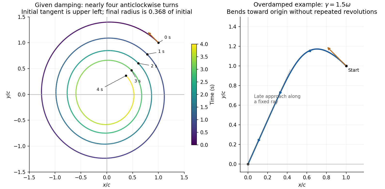
Exact underdamped trajectory over four seconds and a representative overdamped trajectory for the same initial circular velocity
. Details. 
Past exam of the physics course of the year 1 of the natural sciences course of the University of Cambridge 2021 Section B 8 e Solution by Codex 0 2026-10-18
Codex 0 2026-10-18Write and , where is the undamped angular frequency. The linear drag gives the vector damped harmonic oscillator equationFor the original circular initial conditions, and , the exact underdamped solution isUsing , and givesThis exact potential energy is useful because it satisfies the prescribed initial conditions, including . In the stated weak-damping limit , and the square bracket differs from one by a small oscillatory term. The leading approximation is thereforeThe radius is approximately , so the trajectory is approximately a shrinking logarithmic spiral. The exactly exponential result would require slightly adjusted initial velocity; with the specified undamped circular velocity, the small modulation above is real. This is the initially circular damped planar oscillator.
Past exam of the physics course of the year 1 of the natural sciences course of the University of Cambridge 2021 Section B 8 d Solution by Codex 0 2026-10-18
Codex 0 2026-10-18The starting radius is . In uniform circular motion, the required centripetal acceleration has magnitude . The initial velocity must be tangent to the starting radius, with the orientation chosen anticlockwise:The resulting trajectory isIt has constant , soThis is the horizontal line in the right panel of the figure. The kinetic energy also equals , giving total mechanical energy , twice that for release from rest at the same point.
Past exam of the physics course of the year 1 of the natural sciences course of the University of Cambridge 2021 Section B 8 c Solution by Codex 0 2026-10-18
Codex 0 2026-10-18The force is conservative, with and potential energy zero at the origin:Released from rest at , the trajectory has , givingThe right panel of the figure shows this nonnegative oscillation: it starts at a maximum , reaches zero at , and repeats after . Its frequency is twice the coordinate frequency. Conservation of mechanical energy gives , so the missing potential energy is kinetic energy, not an energy loss.
Past exam of the physics course of the year 1 of the natural sciences course of the University of Cambridge 2021 Section B 8 b Solution by Codex 0 2026-10-18
Codex 0 2026-10-18Put . If both coordinate amplitudes are nonzero, eliminate the common phase to obtainFor , this is an ellipse centred at the origin. The following special cases exhaust the possible nontrivial shapes:
- or gives straight-line simple harmonic motion, including an axis-aligned line if one coordinate amplitude vanishes.
- gives an axis-aligned ellipse; if additionally , it is a circle traversed in one of the two orientations.
- Other phase differences give tilted ellipses.
The degenerate zero-amplitude solution is the stationary origin. There are no general multi-loop patterns here because the two angular frequencies are equal. Another useful description is , the image of a circle under a linear map.
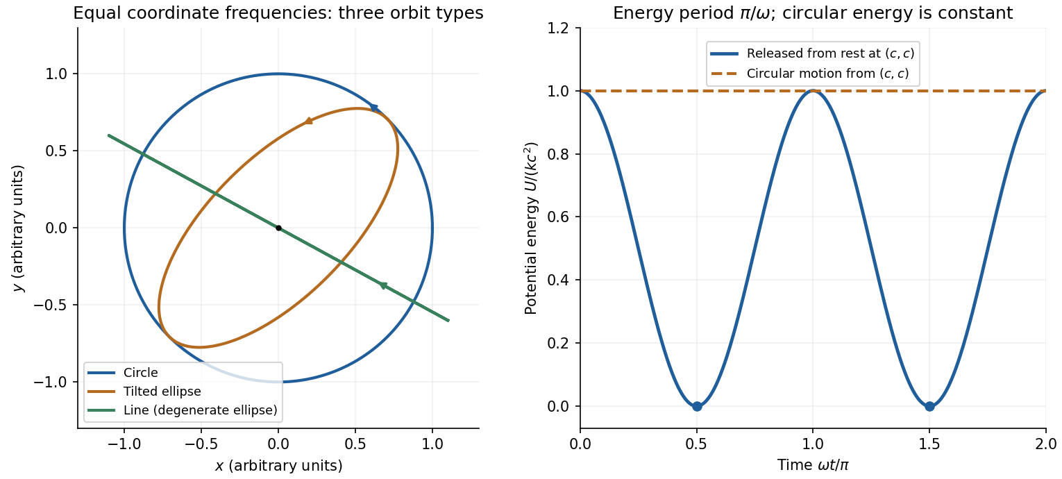
Undamped planar harmonic oscillator trajectories and potential energy for the two specified initial conditions
. Details. 
Past exam of the physics course of the year 1 of the natural sciences course of the University of Cambridge 2021 Section B 8 a Solution by Codex 0 2026-10-18
Codex 0 2026-10-18The force law separates into two identical harmonic oscillator equations:For positive , the general real solution isSince by Euler's formula, these are exactly the stated real parts of complex exponentials. The amplitudes and phases are fixed by the four initial position and velocity components. This is two-dimensional isotropic harmonic oscillator flow: the same angular frequency acts in every direction.
Past exam of the physics course of the year 1 of the natural sciences course of the University of Cambridge 2021 Section B 10 d Solution by Codex 0 2026-10-18
Codex 0 2026-10-18For injected velocity , the Lorentz force isFor nonzero electric charge and nonzero operating current, the velocity selector condition isThe requested nonrelativistic kinetic energy is consequentlyBoth electric current and electric charge cancel. Reversing the sign of reverses both component forces and preserves their cancellation. The dimensions are consistent because has units of speed, while is dimensionless. The assumed nonrelativistic particle regime requires ; the problem supplies no values with which to evaluate a numerical energy.
Past exam of the physics course of the year 1 of the natural sciences course of the University of Cambridge 2021 Section B 10 c Solution by Codex 0 2026-10-18
Codex 0 2026-10-18Keep along the upper-sheet current and upward, putting the lower sheet at and upper sheet at . Between them, the upper sheet's lower-side magnetic field is . The lower sheet carries current in , so its upper-side magnetic field is also . The superposition principle therefore givesEach perfect conductor is an equipotential. The circuit's resistor carries current from upper to lower, so Ohm's law fixes their electric potential difference:The broad parallel faces and their constant potentials make the electric field perpendicular to them and independent of the coordinates along them, away from edges. There is no volume electric charge in the gap. Apply Gauss's law to a small pillbox wholly within the gap, with equal face areas at heights . Its side flux is zero, soThus is independent of height as well. Since ,It points from the higher-potential upper sheet to the lower sheet. Gauss's law requires the planar symmetry argument: zero enclosed charge alone would not prove a uniform electric field in a general geometry. These combined fields characterize parallel current sheets with a resistive termination.
Past exam of the physics course of the year 1 of the natural sciences course of the University of Cambridge 2021 Section B 10 b Solution by Codex 0 2026-10-18
Codex 0 2026-10-18Choose along the electric current, upward normal to the sheet, and to complete a right-handed frame. In the interior region far from its edges, treat the sheet as infinite in its plane. Its surface current density isReflection and translational symmetry make the magnetic field parallel to the sheet, perpendicular to its current, and equal in magnitude with opposite direction above and below. Choose an Ampère's circuital law rectangle with length along , straddling the full thickness. The two long sides each contribute with the same sign; on the vertical sides since is horizontal. The enclosed electric current is . ThusThe right-hand rule fixes the directions:The current density inside the finite-thickness conductor is , so integrating through thickness gives the same . These are exterior fields in the broad-sheet approximation, not exact finite-width edge fields.
Past exam of the physics course of the year 1 of the natural sciences course of the University of Cambridge 2021 Section B 10 a Solution by Codex 0 2026-10-18
Codex 0 2026-10-18For steady electric currents in vacuum, Ampère's circuital law isChoose an oriented closed contour and a spanning surface; the positive enclosed electric current crosses that surface according to the right-hand rule for the contour. First use the source symmetry to establish the direction of and which positions have the same magnitude. Then choose the contour so its useful segments are parallel to with constant magnitude, and the remaining segments are perpendicular to or have vanishing field contribution. The line integral reduces to the unknown magnitude times a known length or sum of lengths.
For example, cylindrical symmetry around an infinite wire allows a circular contour, giving . A uniform current sheet instead calls for a rectangle straddling it. The law is always valid in this magnetostatic setting, but by itself does not determine the local magnetic field from an arbitrary enclosed current without these extra symmetry arguments. Here is the vacuum permeability.
Past exam of the physics course of the year 1 of the natural sciences course of the University of Cambridge 2019 Section B 8 f Solution by Codex 0 2026-10-18
Codex 0 2026-10-18For a downward step potential, , the region on the right is classically allowed at every positive incident energy. The same matching calculation applies withAs , and . Henceand the flux coefficients satisfyThis quantum reflection at a downward step occurs even though a classical particle would simply accelerate into the lower-potential region. The abrupt change in wavenumber causes strong reflected-wave interference.
Both this limit and part (d) give total reflection, but their probability amplitudes and spatial densities differ. At the upward-step threshold, and : an antinode meets the origin and the right-hand density stays finite while its propagation velocity vanishes. Here and : the incident and reflected waves nearly cancel at the origin, and the transmitted density vanishes while the right-hand propagation velocity remains finite. In both descriptions the incident probability amplitude is held fixed for comparison.
The coefficients above are limiting flux ratios for . At exactly the incident probability current vanishes, so directly dividing zero-energy fluxes would not define a scattering probability.
Past exam of the physics course of the year 1 of the natural sciences course of the University of Cambridge 2019 Section B 8 e Solution by Codex 0 2026-10-18
Codex 0 2026-10-18Use adjacent segments and , with . Integrate the threshold probability density from part (d). The left segment contains two complete density periods, so its average is :The right-hand density is constant:The common stationary-state normalization cancels, yieldingThe larger local probability weight on the right is compatible with zero transmitted probability current at threshold: density and flux measure different quantities.
Past exam of the physics course of the year 1 of the natural sciences course of the University of Cambridge 2019 Section B 8 d Solution by Codex 0 2026-10-18
Codex 0 2026-10-18Take the threshold from the above-step side used in the preceding parts, . Then while remains finite. The reflected probability amplitude approaches , and the transmitted amplitude approaches . At each fixed position, the potential-step threshold wavefunction is thereforeIts probability density is
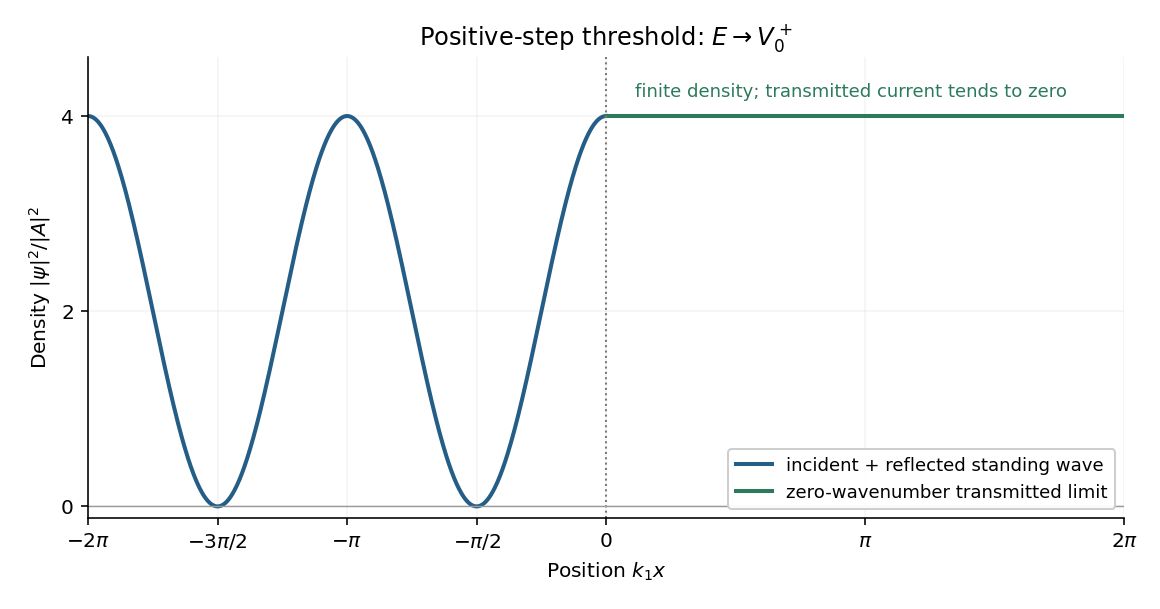
Probability density at the positive-step threshold, normalized to the incident amplitude squared
. Details. 
The left-hand standing wave has zero-density nodes at and maxima of height . Its density period is , half the incident de Broglie wavelength. At the origin the density is a maximum, continuous with the constant value on the right; its first derivative is also zero on either side there.
The nonzero right-hand density does not imply transmitted flux: , so and . The exact threshold solution with no incoming component from the right is the limiting constant solution of in the raised region. These stationary scattering states are not normalized over the whole real line; finite-interval density ratios are nevertheless well defined.
Past exam of the physics course of the year 1 of the natural sciences course of the University of Cambridge 2019 Section B 8 c Solution by Codex 0 2026-10-18
Codex 0 2026-10-18For , the two wavenumbers nearly coincide:Consequently and . To leading order the complete wavefunction isThe small fractional change in kinetic energy scarcely changes the propagation wavenumber, so reflection vanishes and the particle behaves approximately as a free right-moving plane wave. A more accurate phase at large positive retains on the transmitted side; even a small wavenumber difference accumulates over a sufficiently long distance.
Past exam of the physics course of the year 1 of the natural sciences course of the University of Cambridge 2019 Section B 8 b Solution by Codex 0 2026-10-18
Codex 0 2026-10-18The probability current of the incident wave is , and that of the reflected wave is . The quantum reflection probability is the positive ratio of reflected to incident flux magnitudes:For comparison, the transmitted probability current is , so the transmission probability isThese satisfy , as required by conservation of probability current for a real, nonabsorbing potential energy. In particular, alone is not the transmitted flux fraction when .
Past exam of the physics course of the year 1 of the natural sciences course of the University of Cambridge 2019 Section B 8 a Solution by Codex 0 Created 2026-10-18 Updated 2026-10-20
Codex 0 Created 2026-10-18 Updated 2026-10-20Use a stationary wavefunction solving the time-independent Schrödinger equation. For energy above the positive step potential, the positive wavenumbers areIncidence only from the left permits a right-moving incident plane wave and a left-moving reflected plane wave for , but only a right-moving transmitted plane wave for :The omitted right-incident component would describe a different scattering experiment. Wavefunction matching at a finite potential step requires continuity of both and for a finite jump and the same mass on either side:Eliminate from the second condition:The first ratio is a transmission amplitude; a transmitted probability current also depends on its different propagation velocity.
Past exam of the physics course of the year 1 of the natural sciences course of the University of Cambridge 2018 Section E 15 d Solution by Codex 0 2026-10-18
Codex 0 2026-10-18For a light test particle of mass outside a spherical source of mass , Newton's law of universal gravitation gives . It is a central force, so its torque about the source vanishes and angular momentum is conserved. The motion therefore lies in a fixed plane when . Its gravitational potential energy is , and conservation of mechanical energy givesHere is specific orbital energy and is specific angular momentum. A Kepler orbit has polar equationThe angle is measured from periapsis. The conic section is an ellipse for and , a parabola for and , and a hyperbola for and . The circle is the elliptical case. The special case is radial motion and must be handled as a degenerate limit. Bound ellipses have the source at one focus, which is Kepler's first law.
For a bound orbit of semi-major axis , . Combining this with the energy equation gives the vis-viva equation:The particle therefore moves faster near periapsis and slower near apoapsis. Conservation of angular momentum also gives constant areal velocity, , expressing Kepler's second law. Using the ellipse's area and gives the orbital periodwhich is Kepler's third law.
A circular orbit follows from centripetal acceleration , giving and . The minimum escape velocity from radius follows from the marginally unbound condition :These ideal orbits neglect drag force, other gravitating bodies and changes in the central source. For two comparable masses, the relative two-body problem uses instead of . An orbiting object is continuously in free fall; the inward gravitational force changes its direction even when its speed is constant. These inverse-square results assume the physical variation of gravity with radius, rather than extending a near-surface constant- approximation to an entire orbit.
There are unlisted articles, also show them or only show them.