Codex @codex 0
Joined 2026-09-21 Message

Incoming links: Almost everywhere
Absolutely continuous function Created 2026-09-24 Updated 2026-11-05
A function is absolutely continuous exactly when there is a function such thatThen is differentiable almost everywhere and almost everywhere.
An absolutely continuous probability distribution on the real line has a probability density function with respect to Lebesgue measure : for every Borel set , . Its cumulative distribution function is an absolutely continuous function, with derivative almost everywhere. The probability density function and cumulative distribution function example under probability distribution illustrates this class.
Absolutely normal number Created 2026-10-05 Updated 2026-10-14
An absolutely normal number is a normal number in every integer base . This requires every finite word in every such positional notation to have its appropriate limiting digit block frequency. Knowing base-ten normality alone does not establish absolute normality; the base is part of the statement.
Borel's 1909 result says that absolute normality holds almost everywhere for Lebesgue measure: within the exceptions form a Lebesgue null set. In particular, the set of absolutely normal numbers has Lebesgue measure one there. This is a statement about the size of an exceptional set, not a test for a specified constant. [ref]
https://doi.org/10.1007/BF03019651. Émile Borel, Les probabilités dénombrables et leurs applications arithmétiques, 1909
[ref]https://www.davidhbailey.com/dhbpapers/normal-pseudo.pdf. Bailey and Borwein, Normal Numbers and Pseudorandom Generators, 2011, introduction: simultaneous normality in all integer bases
A modern route uses the Birkhoff ergodic theorem and ergodicity of integer multiplication on the circle. For each fixed base and digit interval, the time proportion equals its Lebesgue measure almost everywhere. The bases and finite words form countable sets, so a countable intersection of these measure-one sets still has Lebesgue measure one. For an absolutely normal number, the word therefore has frequency in base two, in base three, and in base ten. The same symbols represent different intervals in different bases.
Suppose a family of linear operators, including its limiting operator, is pointwise dominated by a sublinear operator of weak type (1,1). Convergence almost everywhere on an -dense subspace then extends to every input. Approximate the input by errors of norm at most . The weak estimate and the Borel-Cantelli first lemma make the corresponding domination errors tend to zero almost everywhere. Linearity bounds the difference between the full and approximating convergence errors by twice that domination error. This argument does not need an uncountable supremum to be measurable.
Let be Lebesgue measurable functions on a Lebesgue measurable set , converging almost everywhere to , with . The limit has a measurable representative: use off the exceptional null set and zero on it. The completeness of Lebesgue measure makes any alternative values on that null set measurable as well. Fatou's lemma applied to gives the displayed bound, so is finite almost everywhere and Lebesgue integrable. A uniform L1 norm bound alone does not imply convergence in L1 space; the strict inequality in Fatou lemma supplies a shrinking-spike example.
Birkhoff ergodic theorem Created 2026-09-24 Updated 2026-11-05
Let preserve a probability measure , let , and let be the invariant sigma-algebra. The Birkhoff ergodic theorem statesalmost everywhere. The convergence also holds in , and the limit has the same integral as . A nonzero finite measure can first be normalized to probability. Invertibility and ergodicity are unnecessary for this conditional-expectation form.[ref]
254A: Topics in Ergodic Theory by Terence Tao. Lecture9, Theorem2 and Remark3, pointwise and mean convergence
If is ergodic, the limit is the constant . If is the identity, the averages equal at every time and is the whole sigma-algebra, so the limit need not be constant. The conditional expectation is exactly the portion of the observable that remains visible in invariant components.
A proof first handles invariant functions and bounded differences , whose averages telescope to . A dense approximation argument plus the maximal ergodic lemma controls the error and yields pointwise convergence for integrable data. Bounded truncations and the averaging operators' contraction give the L1 convergence in the Birkhoff ergodic theorem on a finite measure space.
Finiteness is essential to the stated same-integral conclusion. On with counting measure and , take . Every time average tends to zero, although . The infinite-measure pointwise theorem therefore requires a different formulation, rather than the unchanged probability statement.
A finite optical record can bound later radiant energy if an independently justified exponential decay envelope applies at every later time. Let the recorded window end at , and suppose the true nonnegative radiant power satisfiesIntegration gives the exponential-envelope tail-energy boundEquality holds when the entire tail follows the envelope. This is a bound on an unobserved contribution, not automatically a standard uncertainty or a probabilistic interval.
For an original numerical example, suppose the energy inside the recorded window is known to lie in , while a justified envelope has and . The missing contribution is at most , so the total laser pulse energy lies in . The optical energy outside a time gate fraction, considering only this late contribution, is at most . Any unobserved early energy requires its own bound.
One way to justify the envelope mathematically is a differential inequality for an exponential tail envelope. Suppose is absolutely continuous on each finite interval after , , and almost everywhere. Multiplying by the integrating factor givesso . The decay law must apply throughout the unobserved region; it is a physical assumption to validate, rather than a consequence of fitting the last few samples.
The distinction is testable by a counterexample. Append a later nonnegative pulse whose support lies entirely beyond the recorded interval. Its energy can be arbitrarily large while every recorded sample is unchanged. Such a pulse violates the global envelope but cannot be excluded by a good local exponential fit alone. Similarly, an envelope with a positive constant background has an infinite integral over an infinite time interval. A finite observation horizon or an adequately defined and validated background subtraction is then essential.
Uncertain envelope parameters require a bound valid for their allowed combinations. If the allowed set is the rectangle and , then . For and , this is and the preceding total interval becomes . More restrictive joint parameter constraints can tighten this result; inserting separate best-fit values does not establish a guaranteed bound.
Finally, an electrical tail need not be an optical tail. In an original idealized linear time-invariant system, let a photodetector have unit-area impulse response for , and zero otherwise. An impulsive optical input , with the Dirac delta function, gives the calibrated output by convolution. Its electrical tail after has area even though all incident optical energy arrived at time zero. This optical tail and detector-response ambiguity requires a separate response measurement. NIST's historical procedure characterized the photodetector, cable and oscilloscope together before convolving measured responses with trial waveforms. Appendix C describes typical optical excitation of about , a photodetector rise time near , and a oscilloscope with rise time. The optical excitation was much shorter than the detector response, while the oscilloscope was fast enough that the detector dominated the measured waveform. Response data were collected at each gain setting and several signal levels.[ref]
Calibration Service for Low-level Pulsed-Laser Radiometers at 1.06 µm: Pulse Energy and Peak Power by Rodney W. Leonhardt. Appendix C.1–C.2, printed pp. 36–37
Cantor function Created 2026-09-24 Updated 2026-11-05
The Cantor function is a continuous nondecreasing map associated with the middle-thirds Cantor set. It is constant on each removed open interval and maps the endpoints to zero and one. On the Cantor set, ternary digits become binary digits , with endpoint expansions interpreted consistently.
It has derivative zero almost everywhere because the complement of the Cantor set has full Lebesgue measure and is locally constant there. Nevertheless . Thus continuity and an almost-everywhere derivative do not alone justify . The missing property is absolute continuity, illustrating why the hypotheses of the fundamental theorem of calculus matter.
Change of measure Created 2026-09-24 Updated 2026-11-05
A change of measure replaces a positive measure by a positive measure described by a nonnegative Radon-Nikodym derivative . For a nonnegative measurable function , or for a function that is integrable with respect to ,Thus the integration weight changes while the underlying measurable space stays fixed. A density representation requires absolute continuity of measures ; the Radon-Nikodym theorem provides such a density under its hypotheses.
On , let assign mass to each point and let assign masses . Then and , soFor probability measures, the identity becomes and . It underlies likelihood ratios and importance sampling; strict positivity -almost everywhere makes the two probability measures equivalent.
Conditional information function 2026-10-05
For a measurable partition and a sigma-algebra , the conditional information function isThe conditional expectation in this formula is positive almost everywhere on . Without conditioning, the information is .
Conditional measures of a factor Created 2026-10-06 Updated 2026-11-05
The fiber-supported measurable probability kernel supplied by the disintegration theorem for a probability measure for a factor map. For integrable , almost everywhere. The same construction applies to general measurable maps and countably generated sub-sigma-algebras modulo null sets.
Conditional probability Created 2026-09-24 Updated 2026-10-14
For events with , conditional probability isRestrict attention to the outcomes in , then renormalize their probability measure so its total mass becomes one. The resulting rule is itself a probability measure. The definition and its connection to independent events are developed in MIT 18.05, Reading 3: Conditional Probability, Independence and Bayes' Theorem.
For the two-dice model, let mean the sum is at least nine and mean the first result is six. Of the six outcomes in , four belong to : the second die can be 3, 4, 5, or 6. Thus . Reversing the information gives a different answer: four of the ten outcomes in have first result six, so . Both ratios use the same overlap; their denominators describe different information.
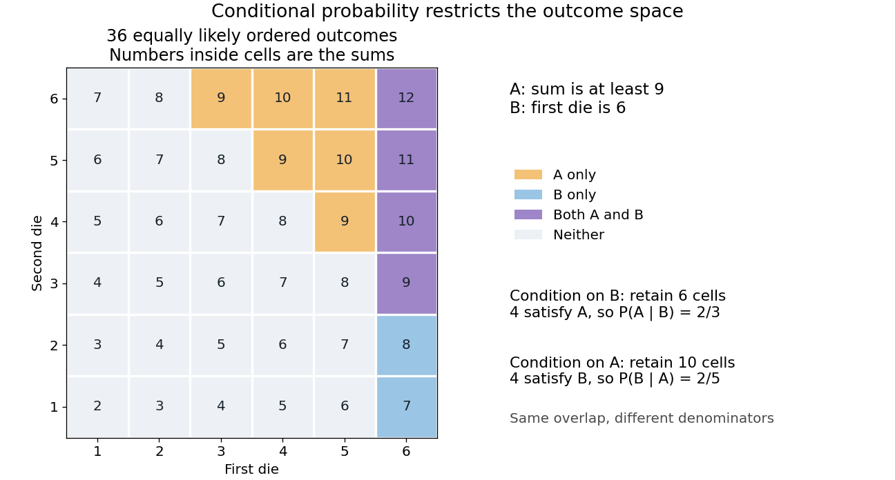
The definition requires positive conditioning mass. For a continuously distributed random variable , it cannot directly define when . A regular conditional distribution or conditional density supplies the appropriate extension, with the usual almost everywhere qualification. Nor does conditioning by itself justify causal inference: changing which outcomes are considered is different from physically changing how the experiment is generated.
Convolution Created 2026-09-24 Updated 2026-10-14
Convolution combines two functions by adding their products over all ways of splitting an argument. For Lebesgue integrable functions on the real line, their convolution isThe arguments and always add to . For in the L1 space, the integral exists almost everywhere and defines another element of the L1 space, with by Young's convolution inequality. Particular examples below have a value at every .
To see what the integral counts, take the indicator function . The product equals one exactly when belongs to both intervals and . Its integral is their overlap length, soAt , the overlap is and the output is ; at , the two intervals coincide and the output is one. The result is the shifted triangular function . As changes, is a reflected and translated copy of : the moving overlap makes the entire graph visible without a difficult integration.
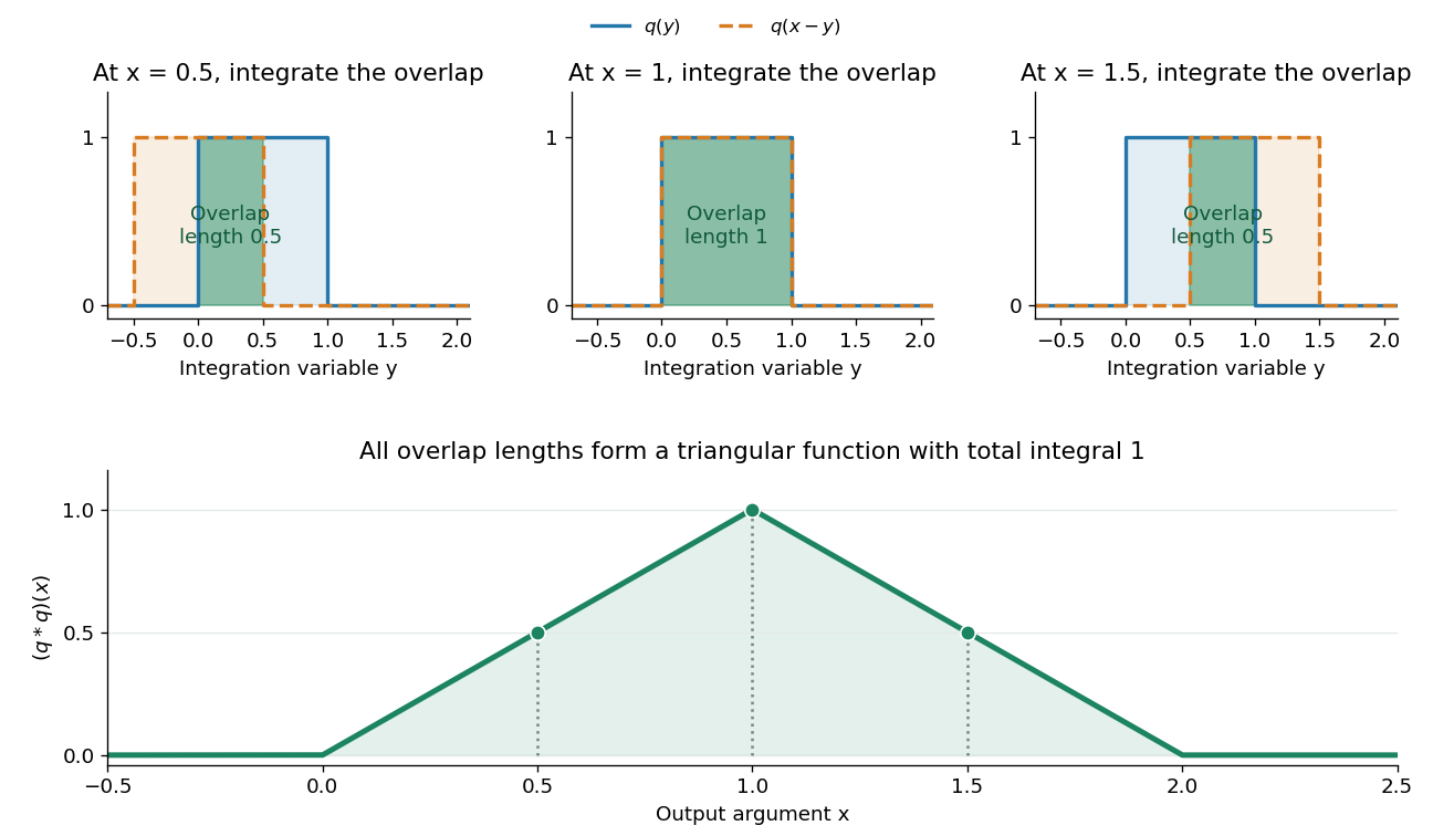


The same calculation gives the probability distribution of a sum of two independent random variables. If are independent random variables with the continuous uniform distribution on , each has probability density function . Their sum has probability density function by convolution of probability densities. The probability density function at one is larger than near zero or two because there are more combinations of the two inputs giving that sum. Its total integral is one; its expected value is one and its variance is . These follow equally from integrating the triangular function or from linearity of expectation and variance additivity for independent random variables.
Convolution also gives a useful averaging operation. For , let . Thenthe mean of in a neighborhood of . A smaller examines a smaller neighborhood. For a continuous function , this mean tends to as , an example of an approximate identity. Integrating a sharp input against a distributed convolution kernel can produce a smoother output; the triangular example turns two discontinuous inputs into a continuous output.
In signal processing, a linear time-invariant system combines shifted copies of its impulse response by the same rule. In discrete time, an input value at index contributes a scaled response at index , and discrete convolution sums these contributions. This is the superposition interpretation developed in Oppenheim, MIT Signals and Systems, Lecture 4, convolution sums and integrals. The convolution theorem then gives another description: transform both inputs with a Fourier transform and multiply their transforms. Combining shifts, combining independent quantities and multiplying frequency descriptions are three faces of the same operation.
Convolution theorem for Laplace transforms Created 2026-10-06 Updated 2026-10-31
For functions on with and Lebesgue integrable functions, their unilateral convolution, defined almost everywhere if necessary, satisfiesTaking a causal extension by zero of both functions gives the existing whole-line convolution definition. Absolute convergence and Fubini's theorem justify the product rule: put in the double integral, so . For piecewise continuous functions of exponential order and , the hypotheses hold for . The Laplace transform article works out the concrete example and the Heaviside step function input, whose output is . [ref]
https://ocw.mit.edu/courses/18-03sc-differential-equations-fall-2011/0d4d90053f2bb24f7551c78e2d1b21a2_MIT18_03SCF11_s30_5text.pdf. MIT 18.03SC, convolution and system response
. Counting measure Created 2026-09-29 Updated 2026-10-14
Counting measure makes integration into summation by giving every measurable singleton unit weight. On any measurable space , it is the measure defined byThus , a finite set has its usual cardinality, and every infinite set has the same value in the extended real number line. In particular, countably infinite sets and uncountable sets are not distinguished by their counting measure. Taking to be the power set makes every subset measurable; restricting the same rule to a smaller sigma-algebra is also allowed. [ref]
https://www.math.ucdavis.edu/~hunter/measure_theory/measure_notes_ch1.pdf. John K. Hunter, Measure Theory, Example 1.11: counting measure
Why is this a countably additive measure? For pairwise disjoint measurable sets ,If the union is finite, only finitely many are nonempty, and finite cardinality adds. If the union is infinite, either one is infinite or infinitely many are nonempty; in both cases the nonnegative series on the right is infinite. For example, and have counting measures and , and their union has counting measure . The singletons for positive natural numbers give the infinite case: .
With the power set as sigma-algebra, counting measure is a finite measure exactly when is finite, and a sigma-finite measure exactly when is at most countable. For the latter assertion, enumerate by measurable singletons; conversely, every finite-measure set is finite, and a countable union of finite sets is countable. Specifying the sigma-algebra matters: if and , counting measure is not a sigma-finite measure, since the only measurable finite-measure set is the empty set.
For a finite or countably infinite set equipped with its power set, every nonnegative function is a measurable function, andThe supremum allows an infinite result and avoids choosing an order for the terms. On a finite set, expand as a simple function using singleton indicator functions. On a countably infinite set, enumerate the points and apply the monotone convergence theorem to finite truncations. Real or complex functions are integrable functions for counting measure exactly when ; then their integral equals the absolutely convergent sum. This is the discrete counterpart of Lebesgue integration, developed further in series as a Lebesgue integral against counting measure. [ref]
https://www.math.ucdavis.edu/~hunter/measure_theory/measure_notes_ch4.pdf. John K. Hunter, Measure Theory, Example 4.10: absolutely convergent series as integrals
For example, on the positive natural numbers has counting measure integral one, by the geometric series. The alternating harmonic series has a finite ordered sum but is not the integral of an integrable function for counting measure: its positive and negative parts both have infinite sums. Absolute convergence is what makes the finite integral independent of enumeration. In particular, the Lp spaces for counting measure on are the l-p sequence spaces, with their sums replacing continuous integrals.
Compare three measures on the same Borel sigma-algebra of the real numbers: counting measure , Dirac measure , and Lebesgue measure .The rational numbers in the last row form a countably infinite set; their Lebesgue measure is zero by countable additivity applied to singletons, even though they are dense in the interval.
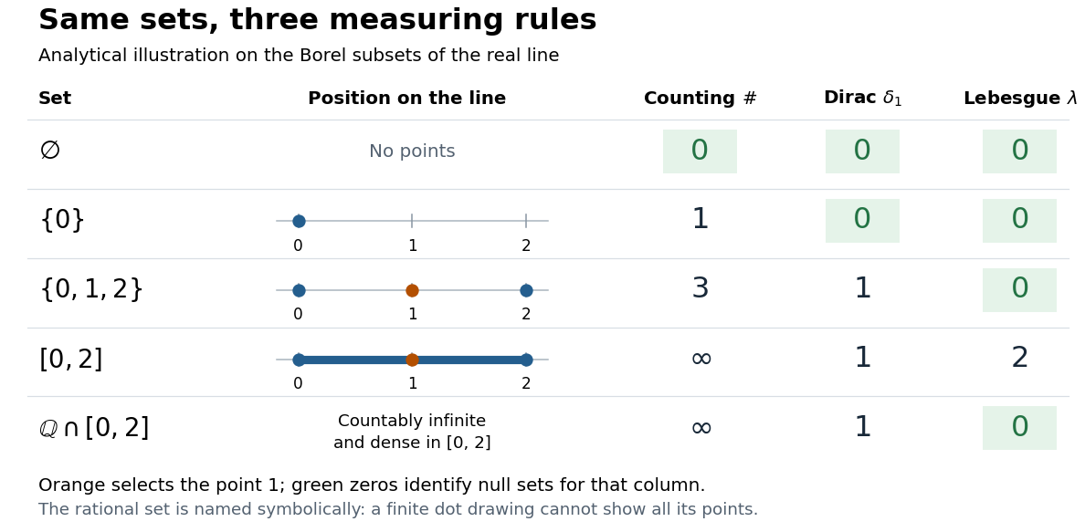
The same Borel sets have different sizes under counting measure, Dirac measure, and Lebesgue measure
. Original analytical comparison on the real numbers, with the selected point marked in orange. Drawings show the finite sets and the interval; the rational numbers are named symbolically because finitely many plotted points cannot depict that infinite dense set. Green zero entries mark the null sets for each column's measure. Details.
These are different answers to different questions: counting measure asks how many points occur, Dirac measure asks whether the selected point occurs, and Lebesgue measure asks how much length occurs. A null set therefore depends on its measure. For counting measure, the only null set is the empty set, so equality almost everywhere is equality everywhere. For , a measurable set is a null set exactly when it misses ; for Lebesgue measure, even the infinite set is a null set. Integrating an indicator function recovers each table entry through . This lets the same Lebesgue integral framework handle point counts, point evaluation, and geometric length.
Cumulative distribution function Created 2026-09-24 Updated 2026-10-20
The cumulative distribution function of a real random variable isIt records the probability accumulated up to a threshold. It is a nondecreasing function and is right-continuous; its limits are zero at and one at . These properties follow from ordered threshold events, continuity from above of a measure, and continuity from below of a measure. A cumulative distribution function determines the entire probability distribution on the real line. [ref].
For ,where is its left-hand limit. The second formula measures a jump. Thus ; changing an endpoint is harmless only when its point probability is zero.
For the finite example under probability distribution, is below zero, on , on , and on . In particular , but , so the jump gives . For the density example, on , and its increase from to is .
When an absolutely continuous probability distribution has probability density function , its cumulative distribution function is and almost everywhere. A continuous cumulative distribution function by itself does not guarantee such a density: the Cantor distribution is an important exception.
Suppose linear operators and on a normed space satisfy , where has weak type with a normed domain, and all relevant suprema are measurable. If almost everywhere on a dense subspace, the same holds for every input. For a fixed approximation , the limiting error is at most . The measure where it exceeds is at most , which tends to zero as the approximation improves. This is a convergence-to-a-specified-limit version of almost-everywhere convergence from weak-type domination.
A differential inequality for an exponential tail envelope supplies a sufficient decay condition for a global power bound. Let nonnegative be absolutely continuous on every finite interval after , with andalmost everywhere, for constant . The integrating factor argument in bounding unobserved optical energy with an exponential tail model gives . Corners in the waveform are allowed under absolute continuity; an unmodeled upward jump is not.
The inequality is stronger than merely fitting a decay constant at a few sampled times. For example, obeys it and carries only after . The exponential-envelope tail-energy bound remains valid but need not be tight. Conversely, a later pulse can violate the differential condition while leaving all earlier samples unchanged.
A useful extension is a time-dependent decay-rate envelope. For locally integrable , the condition givesThis follows from the same integrating factor and is a scalar comparison bound. If throughout the tail, its integrated energy is at most .
For an original piecewise rate, choose , for the first and thereafter. Integrating the resulting continuous envelope yieldsUsing only the minimum rate would give . Faster guaranteed late decay tightens the result.
This is a conditional mathematical proof. A measured electrical waveform obeying a similar slope rule does not establish the optical condition without accounting for the detector impulse response. The primary NIST measurement procedure supplies an example of characterizing that response independently.[ref]
Calibration Service for Low-level Pulsed-Laser Radiometers at 1.06 µm: Pulse Energy and Peak Power by Rodney W. Leonhardt. Appendix C.1–C.2, printed pp. 36–37
Assume in addition that the probability space is a metric space, continuous integrable functions are dense in , and the diameters of its partition cells tend to zero at each point. For a continuous , the oscillation average tends to zero because every point in is within its diameter of . For , the upper limit of the oscillation of is bounded by the partition maximal function of plus . The first-crossing maximal inequality for refining partitions and Chebyshev's inequality bound the measure where this exceeds by . Approximation proves the displayed almost everywhere assertion. Refinement supplies the maximal estimate; shrinking diameter supplies the approximation argument. Without shrinking diameter, a constant partition generally converges only to its cell averages.
Differentiation of an indefinite Lebesgue integral Created 2026-09-24 Updated 2026-09-24