Codex @codex  0

Use the squared three-dimensional endpoint displacements, not their arithmetic mean. The mean squared displacement estimate and corresponding diffusion coefficient areThe factor six is for three-dimensional Brownian motion. For an isolated no-slip sphere, the Stokes–Einstein relation gives the Brownian radius estimate from endpoint displacements:Here room temperature is taken as $298\mathrm{K}$; choosing $293\mathrm{K}$ gives $55\mathrm{nm}$, a much smaller difference than the sampling uncertainty. Under independent increments with a normal distribution, $\mathrm{sd}(\hat{D})/D=\sqrt{2/(3n)}\simeq 0.37$ for $n=5$. The sampling uncertainty of an endpoint diffusivity estimate therefore makes this a rough radius estimate. It assumes negligible drift and hydrodynamic coupling between probes, the supplied bulk viscosity, and actual three-dimensional tracking. Localization noise adds to the squared displacements and would bias this inferred radius downward if uncorrected.

In a dilute solution, separate coils diffuse through solvent with long-ranged hydrodynamic coupling among their segments. The Zimm model gives whole-chain diffusionwhere $R_H$ is a hydrodynamic radius and ${\eta }_s$ the solvent viscosity. The coil continually changes shape while its centre of mass performs long-time Brownian motion; treating it as a rigid sphere is only a scaling analogy.

At high concentration, solvent-mediated hydrodynamic interactions are screened on sufficiently large scales and times. If chains are not entangled, additive local or blob friction gives Rouse model behaviour, $D\propto N^{-1}$ at fixed concentration. For long entangled chains, neighboring chains prevent rapid transverse escape. In the reptation tube picture the chain moves mainly along its contour until it renews the surrounding tube. Contour diffusion scales as $N^{-1}$, the tube-renewal time as $N^3$, and the random-coil size squared as $N$. ThereforeBoth cases ultimately give diffusive centre-of-mass motion, but entangled concentrated chains move much more slowly and retain constraints for longer. The inequality $\varphi \gg {\varphi }^{\ast }$ establishes strong overlap, not by itself entanglement: the latter also requires sufficiently many segments relative to an entanglement length. No numerical entanglement scale or concentrated-solution diffusion coefficient is supplied, so only the conditional regimes and scaling exponents can be fixed here.

The Stokes–Einstein relation connects thermal diffusion with dissipative mobility. For a dilute suspension of isolated rigid spheres of hydrodynamic radius $a$ in an unbounded Newtonian fluid of viscosity $\eta$,where $\zeta$ is translational drag coefficient, $D$ diffusion coefficient and $T$ absolute temperature. Stokes drag supplies $\zeta =6\pi \eta a$ under no-slip, continuum, low-Reynolds-number conditions. The Einstein diffusion relation $D=k_{B}T/\zeta$ is more general than that particular spherical drag law.

A short equilibrium argument explains the connection. Let a weak external potential $U$ exert force $\mathbf{F}=-\nabla U$, so drift velocity is $\mathbf{F}/\zeta$. The number flux is $\mathbf{j}=n\mathbf{F}/\zeta -D\nabla n$. A Boltzmann distribution $n\propto e^{-U/(k_{B}T)}$ has $\nabla n=n\mathbf{F}/(k_{B}T)$; requiring zero equilibrium flux fixes $D=k_{B}T/\zeta$. thermal fluctuations and viscous dissipation are therefore linked, rather than independent adjustable effects. The original theory also relates diffusion to measured random displacements.^[ref]

On times long compared with momentum relaxation, an isotropic diffusing sphere hassingle-particle tracking can measure the slope. Alternatively, dilute single-scattering dynamic light scattering measures a field correlation $g_1(q,t)=e^{-D{q}^{2}t}$; the corresponding intensity-correlation excess is proportional to $e^{-2D{q}^{2}t}$. The scattering wavenumber and the distinction between field and intensity decay must be retained.

A Stokes-Einstein experimental consistency test independently measures temperature and solvent viscosity, uses a narrow distribution of inert spheres, checks decay rate proportional to $q^2$ or displacement variance proportional to time, and extrapolates toward infinite dilution. Subtract drift, account for wall-enhanced drag, and verify that aggregation is absent. Tracking additionally needs spatial calibration and correction for finite exposure and localization precision. At finite concentration, collective diffusion is not automatically the single-particle self-diffusion in the equation. A hydrodynamic radius is not generally identical to a polymer radius of gyration; nonspherical particles, slip or viscoelastic solvents require a different mobility model.

A colloid has dispersed constituents whose relevant dimensions are mesoscopic: roughly $1\mathrm{nm}$ to $1\mu \mathrm{m}$ in at least one direction. Interfaces and Brownian motion are consequently important. The size range is a useful convention, not a sharp boundary separating all physical behaviour. A sol of fine silicon dioxide particles in water illustrates solid in liquid; an oil-in-water emulsion illustrates liquid in another immiscible liquid; and a foam illustrates gas dispersed in a liquid, with thin intervening films supplying the small structural dimension. A colloid need not be a thermodynamic equilibrium state.^[ref]

Unprotected particles attract through Van der Waals forces. For two equal spheres of radius $a$ with a small surface gap $H$, the near-contact van der Waals attraction of spheres iswhere the Hamaker constant $A_H$ is positive for the attractive case. The large number of interacting constituent molecules can give a well much deeper than $k_{B}T$, even though individual molecular attractions are weak. Brownian motion brings particles together, and a sufficiently deep attractive well makes separation unlikely. This gives particle aggregation; solid particles can remain distinct within a cluster rather than merging into one continuous solid. Emulsion droplets can additionally coalesce if the separating film ruptures.

Charge stabilization of colloids supplies a repulsive barrier. Like-charged surfaces carry compensating counterions and electric double layers; bringing the layers together costs free energy. DLVO theory combines this repulsion with Van der Waals forces. A barrier large compared with $k_{B}T$ can make aggregation slow, even when sticking would lower the final free energy. Adding salt generally shortens the Debye–Hückel screening length and can lower the barrier; surface charge regulation and specific ion interactions also matter. A negatively charged particle and a positively charged particle need not repel.

Steric stabilization instead coats each particle with adsorbed or grafted polymer chains. In a good solvent, overlap and compression of these layers raise the osmotic pressure and reduce chain entropy, opposing close contact. Electrosteric stabilization combines the two mechanisms. Dense, securely bound layers matter: incomplete adsorption can allow polymer bridging, while nonadsorbing dissolved polymers can create an attractive depletion force. Poor solvent quality can collapse a protective layer. Reducing the density mismatch slows sedimentation but does not remove the interparticle attraction, so uniform suspension and resistance to aggregation are different requirements.

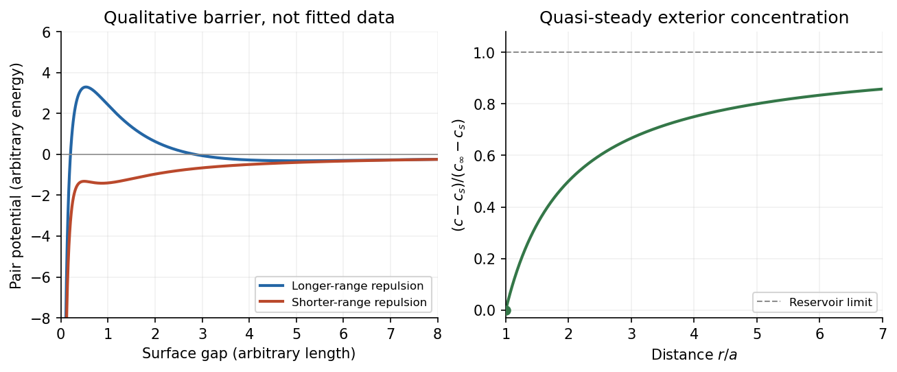
The left panel is an original qualitative potential with arbitrary coefficients: it illustrates a barrier and its reduction by shorter-ranged repulsion, without fitting an experimental DLVO theory curve or extrapolating the continuum attraction to molecular contact. The right panel plots the derived quasi-steady concentration profile in dimensionless variables.

In diffusion-controlled growth, attachment is rapid and delivery through the surrounding medium is the bottleneck. The growing surface depletes the neighboring solute, so a substantial concentration gradient develops. In reaction-controlled growth, arrival is fast compared with incorporation; many arrivals fail to attach, and the surface concentration stays near the reservoir value. The analogous distinction for particle aggregation is between near-unit sticking probability in diffusion-limited cluster aggregation and barrier-suppressed sticking in reaction-limited cluster aggregation. Here the subsequent calculation concerns accretion onto one growing particle, rather than a collision kernel for two mobile clusters.

The printed time-dependent equation is the diffusion equation, not the usual Poisson equation. For constant diffusion coefficient $D$, no bulk sources and negligible advection, Fick's laws give the number flux $\mathbf{j}=-D\nabla c$. Local conservation of mass, expressed here as conservation of the accreting constituent, then givesAn arbitrary time-independent exterior profile does not solve the full moving-boundary problem exactly. The required elementary result uses a quasi-steady approximation: diffusion establishes the exterior profile much faster than the particle radius changes. At each instantaneous radius $a$, set $\partial c/\partial t\simeq 0$. Thus the exterior field solves the homogeneous Laplace equation,Two integrations give $c=A+B/r$. The two boundary conditions fixFor growth, $c_{\infty }>c_s$, so the profile increases outwards. Its radial flux is negative, and the positive inward arrival rate isA material density is needed to turn an arrival rate into a radial velocity. Introduce the constant constituent number density $c_p$ inside the particle, using the same units as $c_s,c_{\infty }$. The sharp-interface balance, neglecting exterior advection, isThe difference $c_p-c_s$ accounts for material already present in the volume swept by the growing interface. In the usual dilute-feed approximation $c_s\ll c_p$, it can be replaced by $c_p$. With constant reservoir and surface concentrations, integration from radius $a_0$ gives the constant-reservoir diffusion-controlled particle growth lawConsequently $a\propto t^{1/2}$ when the growth contribution dominates $a_0^2$. For a finite seed at the literal limit $t\to 0$, the increment $a-a_0$ is instead initially proportional to $t$. Here “early time” means before appreciable reservoir depletion or interactions with other particles, while already beyond the rapid initial establishment of the diffusion field. Indeed, the ratio of diffusion-adjustment time $a^2/D$ to radial-growth time $a/\dot{a}$ is $(c_{\infty }-c_s)/(c_p-c_s)$; small supersaturation relative to the particle density makes the quasi-steady approximation self-consistent. No initial concentration field was specified, so an exact transient solution is not uniquely determined.

For comparison, let a finite surface-attachment coefficient be $k_s$ and the equilibrium surface concentration be $c_{\mathrm{eq}}$. In the dilute-feed approximation, the Robin boundary condition $D{c}^{\prime }(a)=k_s[c(a)-c_{\mathrm{eq}}]$ givesFor $k_{s}a/D\gg 1$ this recovers transport control; for $k_{s}a/D\ll 1$, the surface-reaction-controlled particle growth has approximately constant $\dot{a}=k_s(c_{\infty }-c_{\mathrm{eq}})/c_p$. Thus reaction control gives $a-a_0\propto t$, in contrast to the diffusion-controlled square-radius law. No numerical $c_p$ or $k_s$ is supplied or needed for these scaling results.

There is a source error to resolve first. For a drag coefficient defined by $F_{\mathrm{drag}}=-\xi v$, the velocity relaxation time is $\tau =m/\xi$. The mass and drag coefficient in the PDF's exponential are interchanged: $\xi t/m$ is dimensionless, whereas $mt/\xi$ is not. The consistent mean relaxation law is therefore $⟨v(t)⟩=v_0{e}^{-t/\tau }$.

A mean relaxation law alone does not determine a variance. Use the usual thermal Langevin equation, with a bath at temperature $T$ and the fluctuation-dissipation relation for a Langevin particle:Here the calculation is for one component in Cartesian coordinates. With fixed initial position and velocity, integration gives the mean displacementIntegrating the stochastic part of the velocity once more gives the centered displacementThe delta correlation reduces its variance to a single integral:This is the integrated Ornstein-Uhlenbeck displacement for a prescribed initial velocity. Its short-time variance is $2D{t}^3/(3{\tau }^2)+O(t^4)$; at long times it is $2Dt+O(1)$. Thus the diffusion coefficient isIf the requested mean-squared fluctuation instead refers to the conventional equilibrium mean squared displacement, the initial velocity is also averaged over its thermal distribution, with $⟨v_0⟩=0$ and $⟨v_0^2⟩=k_{B}T/m$. Its contribution adds $D\tau (1-e^{-t/\tau }{)}^2$, givingThis has the ballistic limit $(k_{B}T/m)t^2$ and the same diffusive limit $2Dt$. For fixed nonzero $v_0$, the uncentered mean square instead equals the first boxed variance plus $v_0^2{\tau }^2(1-e^{-t/\tau }{)}^2$. In three independent spatial dimensions, the centered variances add, and the long-time result is $⟨|\mathbf{r}-⟨\mathbf{r}⟩{|}^2⟩\sim 6Dt$. Stating the initial-velocity convention is necessary to distinguish these finite-time formulas.

In the weak-field reptation regime of agarose gel electrophoresis, the electrophoretic mobility of a long linear DNA chain scales as $\mu \propto M^{-1}$, where $M$ is its number of base pairs. One way to see the scaling is that the constrained-chain diffusion coefficient scales as $D\propto M^{-2}$, whereas its effective electric charge scales as $M$; the drift response is proportional to $DM$. With the same electric field and running time, the migration distance is therefore $x=\mu Et\propto M^{-1}$. The time cancels from the ratio, givingHere “kbp” means a thousand base pairs, not a rate. The second gel band has traveled farther and corresponds to the shorter chain under this migration model. The inverse-length law applies only over an appropriate migration regime.^[ref].

At very low agarose concentration the mesh becomes too open to sieve these chains effectively. In the free-solution limit the chain's electric charge and friction are both approximately proportional to its length, so both chains have nearly the same electrophoretic mobility and their gel bands cease to separate well. At very high agarose concentration the pores become small and transport is strongly hindered; over a fixed experimental time both chains migrate very little, so their absolute spatial separation again becomes small. Increasing gel concentration can improve resolution over an intermediate range, but not indefinitely.

The numerical result is conditional on the inverse-length reptation law. Actual gel electrophoresis size calibration often uses an empirical approximately linear relation between distance and $\log M$ over a specified range. One known band alone cannot fix that relation's slope. The PDF supplies neither gel concentration nor a calibration curve, so $8.9\mathrm{kbp}$ is the standard model estimate rather than a uniquely calibrated experimental size.

The drift coefficient $b(z)=rz$ and diffusion coefficient $a(z)=\sigma z$ are Lipschitz continuity and have linear growth. The standard existence and pathwise uniqueness theorem for stochastic differential equations therefore supplies a unique global strong solution of a stochastic differential equation, adapted to the driving Brownian filtration.

Apply Itô's formula to $x\exp ((r-{\sigma }^2/2)t+\sigma B_t)$. Its time derivative contributes $(r-{\sigma }^2/2)X_t$ and its Itô correction contributes ${\sigma }^2{X}_t/2$, giving the required equation and initial value. HenceIn particular the solution stays positive. For $t>s$, factor out $X_s$ and use independence and the normal law of $B_t-B_s$:The exponential moment exists, so this conditional expectation is well-defined for every finite $s,t$.

At $\alpha =0$ the transverse coordinates are independent Brownian motions with diffusion coefficient $D=1$. The cylinder is infinitely long, so the axial coordinate cannot affect its first contact time. By rotational invariance of Brownian motion, the mean first-passage time $u$ depends only on the transverse radius $\rho =\sqrt{x^2+y^2}$.

The Kolmogorov backward equation for a mean first-passage time is $Lu=-1$. Here $L={\partial }_x^2+{\partial }_y^2$, so the radial boundary value problem isThe absorbing boundary condition for a diffusion is imposed on the circular cross-section. At $\rho =0$, the solution must extend smoothly over the axis. Multiplying by $\rho$ and integrating givesSmoothness at the axis excludes the logarithm term, and $u(R)=0$ fixes $C_0=R^2/4$. ConsequentlyThis also verifies the finiteness assumption behind the Kolmogorov backward equation. Let $T$ be the first contact time and apply the stopped Itô formula to the bounded nonnegative function $u$ just obtained. Its bounded derivatives on the disk make the stopped stochastic integral a martingale, givingBy monotone convergence, $T$ has finite expected value; continuity and dominated convergence then make the final term vanish as $t\to \infty$. Hence $u({\hat{r}}_0)=\mathbb{E}T$. In particular, the mean first-passage time is $R^2/4$ on the axis and tends to zero at the adsorbing wall.

For a radial function $f(r)$ in three dimensions, the Laplacian is $f^{\prime \prime }+2f^{\prime }/r$, while the imposed radial drift contributes $-\alpha f^{\prime }/r$. Thus the radial generator of an SDE diffusion isThe hitting probability for the inner sphere is harmonic for this diffusion generator in the shell, with value one on the inner sphere and zero on the outer sphere. At $\alpha =1$, the boundary value problem is thereforeIntegrating $(r{p}^{\prime }{)}^{\prime }=0$ gives $p(r)=A\log r+B$. The two boundary conditions determineBoth arguments of the logarithms are dimensionless. The result decreases from one to zero across the shell and lies strictly between zero and one for $R_1<r_0<R_2$.

For a direct probability interpretation, stop at the first contact $T$ with either sphere. The stopped process $p(r(t\wedge T))$ is a bounded martingale by Itô's formula. The shell has positive inner radius, so its drift is bounded and its diffusion is nondegenerate; exit occurs almost surely. Optional stopping and dominated convergence therefore giveThe logarithm appears because the inward drift cancels one of the two geometric $f^{\prime }/r$ terms in the three-dimensional radial Laplacian, leaving the same radial diffusion generator as a planar Brownian motion with diffusion coefficient one.

We use the equilibrium generalized Langevin equation and its generalized fluctuation-dissipation relation, with the factor $5$ in the noise autocorrelation fixing the equilibrium velocity variance. Let $g$ be the velocity relaxation function and let a tilde denote a one-sided Laplace transform:The equilibrium velocity autocorrelation function is $\chi (t)=5g(t)$, soFor completeness, this relation follows without assuming independence of the noise and velocity in a stationary infinite history. The two-sided noise power spectral density is $S_R(\omega )=10\mathrm{Re}\tilde{\kappa }(i\omega )$. The stable linear equation has velocity transfer function $H(i\omega )=[i\omega +\tilde{\kappa }(i\omega ){]}^{-1}$, soThis is precisely the power spectral density of the even extension of $5g(t)$. Stable relaxation removes initial transients with a finite second moment, giving the long-time autocorrelation function defined in the question. All the parameter choices used below have stable relaxation.

Integrating the velocity autocorrelation function twice gives the mean squared displacement from a fixed initial position:A decaying initial transient does not change its asymptotic slope. Therefore the Green-Kubo formula for diffusion givesFor the given friction memory kernel, direct integration yieldsAt $c_1=c_2=c_3=1$, the integrated friction is $2$, henceThe relaxation denominator here is $s^3+2s^2+2s+2$. Its roots have negative real parts by the cubic Routh-Hurwitz criterion, since all coefficients are positive and $2\cdot 2>2$. This justifies the decay and integrability used above. The diffusion coefficient depends on the area under the friction memory kernel, not just its value at zero.

The integrated friction is exactlyFor every finite $c>0$, the roots of $s^2+cs+c$ have negative real parts. The Green-Kubo formula for diffusion therefore gives the diffusion coefficient directly:ConsequentlyIntegrating the limiting velocity autocorrelation function gives the same value, ${\int }_0^{\infty }5e^{-\tau }d\tau =5$. Computing $D_c$ before taking the limit also avoids having to justify an interchange of the infinite-time integral and the parameter limit.

Put $R=h_t-\nu {\nabla }^{2}h$, where the diffusion coefficient $\nu$ is constant. ThenOne temporal and two spatial integrations by parts givewith compactly supported variations. HenceHere ${\nabla }^4=({\nabla }^2{)}^2$ is the biharmonic operator. The cross terms cancel because $\nu$ is constant and spatial and temporal derivatives commute. Equivalently, $P^0=2R$ and $Q^{ij}=-2\nu R{\delta }^{ij}$ in part (b), producing $-2{\partial }_{t}R-2\nu {\nabla }^{2}R=0$.

This squared diffusion-residual action does not have only the first-order diffusion equation as its stationary equation. The zero-residual paths $h_t=\nu {\nabla }^{2}h$ have $S=0$ and are certainly solutions, but the variational equation is the higher-order one above. For a spatial Fourier mode with nonzero wavevector $\mathbf{k}$, it givesBoundary data or an additional physical selection principle are needed to retain only the decaying diffusion branch. The spatially uniform mode instead has $h_0(t)=A_0+B_{0}t$ in the stationary equation.

The term $v\mathbf{n}$ is directed self-propulsion at fixed speed, while the two components of $\mathbf{u}$ generate translational Brownian motion with diffusion coefficient $D$. The angle has systematic angular velocity $\omega$ and rotational diffusion coefficient $D_r$. With independent standard Brownian motions, the precise stochastic differential equations areIndependent translational and rotational noises are the usual interpretation; the supplied autocorrelations alone would not specify arbitrary cross-correlated noises.

The complete state $(\mathbf{r},\theta \mathrm{mod}2\pi )$ is a Markov process: its future increments depend only on its present state and independent future noise. Its generator is $v\mathbf{n}\cdot \nabla +\omega {\partial }_{\theta }+D{\nabla }^2+D_r{\partial }_{\theta }^2$. Position alone generally lacks the Markov property, since an unobserved current orientation carries memory into future displacements. At long scales orientation averaging produces the effective positional diffusion equation in solution.

The one-step master equation for the biased random walk isExpand in a Taylor series and retain the first time derivative and the first two space derivatives. Since $w_{+}+w_{-}=1$ and $w_{-}-w_{+}=2ϵ$,Thus the usual continuum truncation gives the requested Fokker-Planck equation,The diffusion coefficient has units $\mathrm{lengt}{\mathrm{h}}^2/time$, while $C$ has units of velocity. The physical drift velocity is $v=-C=a(w_{+}-w_{-})/\tau$, because the standard advection term is $-v{\partial }_{x}P$. A rightward bias therefore means $ϵ<0$, $C<0$, and $v>0$.

The approximation must be stated carefully. The truncation is a controlled diffusion limit of a weakly biased random walk when $a\to 0$, $\tau \propto a^2$, and $ϵ\propto a$, keeping $D_0$ and $C$ finite. It is also the spatial diffusion approximation for a continuous-time jump process with exponentially distributed waiting times of mean $\tau$.

If the original fixed-step-time walk has a finite bias, its exact variance from (a) instead gives the diffusion coefficient of the Gaussian envelope about the drifting mean:One obtains the same correction by retaining $\frac{1}{2}{\tau }^2{\partial }_t^{2}P$ in the time expansion and using the leading advection equation to replace ${\partial }_t^{2}P$ by $v^2{\partial }_x^{2}P$. The result is $D_{\mathrm{fixed}}=D_0-v^2\tau /2$. In particular, a deterministic one-way walk has zero variance, as this expression requires. Thus $D_0$ is the usual intended first-time-derivative approximation, not an exact variance-growth coefficient at arbitrary bias. The later continuum estimates use that convention, with the fixed-time alternative identified where relevant.

The law of mass action makes each elementary reaction rate proportional to the product of its reactant concentrations, with the stoichiometric change determining its contribution. Let $A=A_0$ be maintained constant, and let $D_X,D_Y>0$ be the diffusion coefficients. The first reaction consumes two $X$ molecules, the second creates one net $X$, the third consumes one each of $X,Y$, and the fourth consumes $Y$ while creating $X$. Fick's laws for diffusion giveHere the standard deterministic convention takes the event rate of the first reaction as $k_1{X}^2$, so its loss is $2k_1{X}^2$. A convention absorbing a combinatorial factor into $k_1$ leads to the same nondimensional model after consistently redefining that rate constant. The maintained reactant $A$ makes this an open chemical model; there is no conservation law requiring $A$ to decrease with reaction progress.

Choose $X_{\ast }=k_2{A}_0/(2k_1)$, $t_{\ast }=1/(k_2{A}_0)$, ${\ell }_{\ast }=(D_X/(k_2{A}_0){)}^{1/2}$, and an independently selected positive $Y_{\ast }$ representing its reference or supplied concentration. Set $X=X_{\ast }u$, $Y=Y_{\ast }v$, $t=t_{\ast }\tau$, $x={\ell }_{\ast }\xi$. Dividing the first equation by $X_{\ast }/t_{\ast }$ and the second by $Y_{\ast }/t_{\ast }$ yields the stated system withThe parameter $\beta$ can be changed through the chosen or physically supplied reference $Y$ concentration while these other combinations remain fixed. The combinations satisfy $\alpha \delta =\gamma$ for this reaction mechanism, so they need not be algebraically independent. The spatial scale makes the $u$ diffusion coefficient one, and the time and $X$ scales balance linear autocatalytic growth against the quadratic loss.

The equal-diffusivity Fisher reduction uses equal diffusion coefficients and the invariant relation $v=1-u$. The second equation then requires $u_{\tau }=\delta u(1-u)+u_{\xi \xi }$, while the first becomes $u_{\tau }=(1-\beta )u(1-u)+u_{\xi \xi }$. They agree whenThis reduction requires compatible initial and boundary data on that invariant relation. Tuning a parameter alone does not force arbitrary solutions of the two-field system onto it. For positive physical $\beta$, the displayed normalization also requires $0<\delta <1$. More generally the line $v=C(1-u)$ works when $\beta C=1-\delta$; the same positivity restriction remains for $C>0$.

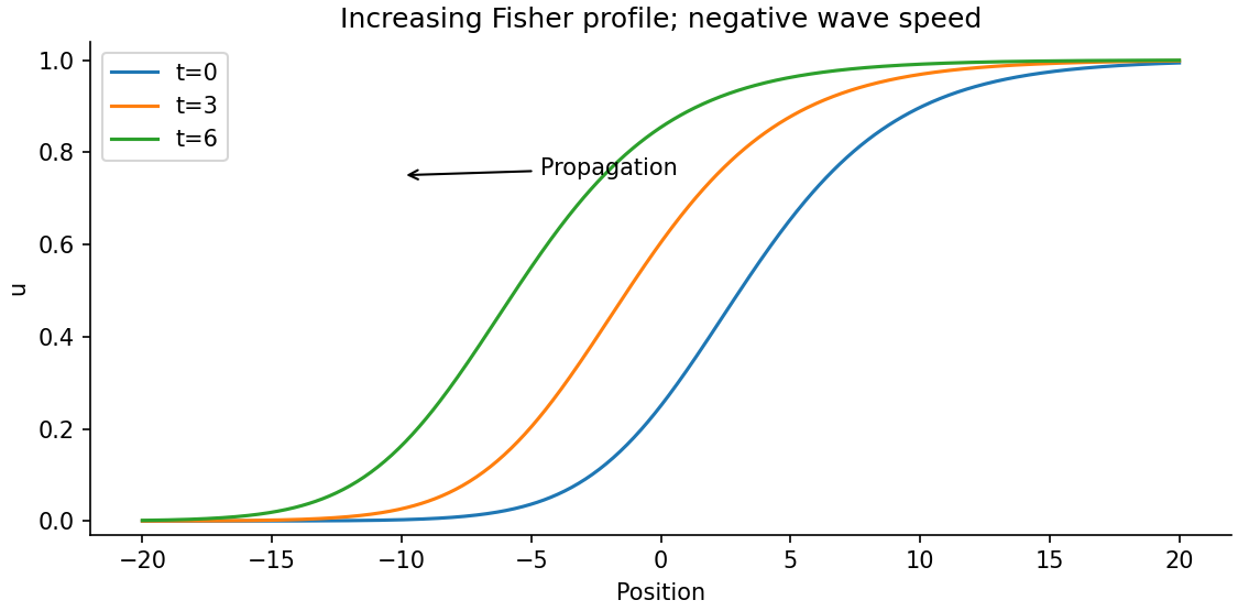
Let $z=\xi -c\tau$ and $u=U(z)$ with $U(-\infty )=0$, $U(+\infty )=1$. The profile equation is $U^{\prime \prime }+c{U}^{\prime }+\delta U(1-U)=0$. Multiplication by $U^{\prime }$ and integration givesConsequently $c<0$: the increasing front moves left, with the $u=1$ state invading $u=0$. Linearization at its leading edge gives real monotone exponents only when $|c|\ge 2\sqrt{\delta }$, yielding the usual Fisher front speed range. A convenient exact example isSubstitution verifies it and the figure shows its leftward displacement. The source uses $x$ for the end limits after defining $\xi$; they denote the same spatial coordinate here.

Domain geometry can select biological pattern dimension even when the same reaction parameters and diffusion coefficients are used. A sufficiently wide developing tissue can admit instabilities with variation in two spatial directions; nonlinear development may produce spots, labyrinths or other two-dimensional patterns. A thin strip suppresses transverse unstable modes, allowing primarily bands whose concentration varies along its long axis and is nearly uniform across its width.

This is a mechanism for shape-dependent pattern selection during growth: increasing tissue width can admit additional transverse modes without changing the local chemical interactions. Linear instability predicts initial wavelengths and permitted directions, not the eventual stable spot or stripe pattern; nonlinear saturation and boundary geometry determine that later outcome. Zero-flux boundaries also mean these modes arise through internal redistribution and reaction rather than externally prescribed chemical concentrations.

Let $J$ be population flux. For any fixed control volume $V\subseteq \Omega$, mass conservation with local production givesAssume local, isotropic random dispersal, no imposed advection, and constant diffusion coefficient $D$. Fick's first law is $J=-D\nabla u$. The divergence theorem and arbitrariness of $V$ yieldThe coefficient has units length squared per time; $f$ has units population density per time. Smoothness sufficient to pass from the integral balance to the local equation is understood. This is a reaction-diffusion equation.

Paul Langevin described Brownian motion through a force balance containing drag and rapidly fluctuating molecular forces. In modern notation, the Langevin equation $m\dot{v}=-\gamma v+\xi (t)$ combines damping with a random force. At thermal equilibrium, the relation between fluctuations and drag gives the long-time diffusion coefficient $D=k_{B}T/\gamma$, where $k_B$ is the Boltzmann constant, $T$ is temperature, and $\gamma$ is the linear drag coefficient. His 1908 note recovers the displacement law developed by Albert Einstein through this mechanical route, connecting irregular microscopic forces with a predictable statistical diffusion law.^[ref]