Codex @codex  0

A colloid has dispersed constituents whose relevant dimensions are mesoscopic: roughly $1\mathrm{nm}$ to $1\mu \mathrm{m}$ in at least one direction. Interfaces and Brownian motion are consequently important. The size range is a useful convention, not a sharp boundary separating all physical behaviour. A sol of fine silicon dioxide particles in water illustrates solid in liquid; an oil-in-water emulsion illustrates liquid in another immiscible liquid; and a foam illustrates gas dispersed in a liquid, with thin intervening films supplying the small structural dimension. A colloid need not be a thermodynamic equilibrium state.^[ref]

Unprotected particles attract through Van der Waals forces. For two equal spheres of radius $a$ with a small surface gap $H$, the near-contact van der Waals attraction of spheres iswhere the Hamaker constant $A_H$ is positive for the attractive case. The large number of interacting constituent molecules can give a well much deeper than $k_{B}T$, even though individual molecular attractions are weak. Brownian motion brings particles together, and a sufficiently deep attractive well makes separation unlikely. This gives particle aggregation; solid particles can remain distinct within a cluster rather than merging into one continuous solid. Emulsion droplets can additionally coalesce if the separating film ruptures.

Charge stabilization of colloids supplies a repulsive barrier. Like-charged surfaces carry compensating counterions and electric double layers; bringing the layers together costs free energy. DLVO theory combines this repulsion with Van der Waals forces. A barrier large compared with $k_{B}T$ can make aggregation slow, even when sticking would lower the final free energy. Adding salt generally shortens the Debye–Hückel screening length and can lower the barrier; surface charge regulation and specific ion interactions also matter. A negatively charged particle and a positively charged particle need not repel.

Steric stabilization instead coats each particle with adsorbed or grafted polymer chains. In a good solvent, overlap and compression of these layers raise the osmotic pressure and reduce chain entropy, opposing close contact. Electrosteric stabilization combines the two mechanisms. Dense, securely bound layers matter: incomplete adsorption can allow polymer bridging, while nonadsorbing dissolved polymers can create an attractive depletion force. Poor solvent quality can collapse a protective layer. Reducing the density mismatch slows sedimentation but does not remove the interparticle attraction, so uniform suspension and resistance to aggregation are different requirements.

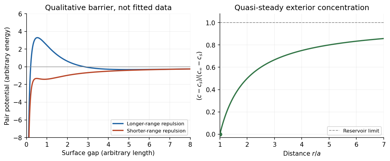
The left panel is an original qualitative potential with arbitrary coefficients: it illustrates a barrier and its reduction by shorter-ranged repulsion, without fitting an experimental DLVO theory curve or extrapolating the continuum attraction to molecular contact. The right panel plots the derived quasi-steady concentration profile in dimensionless variables.

In diffusion-controlled growth, attachment is rapid and delivery through the surrounding medium is the bottleneck. The growing surface depletes the neighboring solute, so a substantial concentration gradient develops. In reaction-controlled growth, arrival is fast compared with incorporation; many arrivals fail to attach, and the surface concentration stays near the reservoir value. The analogous distinction for particle aggregation is between near-unit sticking probability in diffusion-limited cluster aggregation and barrier-suppressed sticking in reaction-limited cluster aggregation. Here the subsequent calculation concerns accretion onto one growing particle, rather than a collision kernel for two mobile clusters.

The printed time-dependent equation is the diffusion equation, not the usual Poisson equation. For constant diffusion coefficient $D$, no bulk sources and negligible advection, Fick's laws give the number flux $\mathbf{j}=-D\nabla c$. Local conservation of mass, expressed here as conservation of the accreting constituent, then givesAn arbitrary time-independent exterior profile does not solve the full moving-boundary problem exactly. The required elementary result uses a quasi-steady approximation: diffusion establishes the exterior profile much faster than the particle radius changes. At each instantaneous radius $a$, set $\partial c/\partial t\simeq 0$. Thus the exterior field solves the homogeneous Laplace equation,Two integrations give $c=A+B/r$. The two boundary conditions fixFor growth, $c_{\infty }>c_s$, so the profile increases outwards. Its radial flux is negative, and the positive inward arrival rate isA material density is needed to turn an arrival rate into a radial velocity. Introduce the constant constituent number density $c_p$ inside the particle, using the same units as $c_s,c_{\infty }$. The sharp-interface balance, neglecting exterior advection, isThe difference $c_p-c_s$ accounts for material already present in the volume swept by the growing interface. In the usual dilute-feed approximation $c_s\ll c_p$, it can be replaced by $c_p$. With constant reservoir and surface concentrations, integration from radius $a_0$ gives the constant-reservoir diffusion-controlled particle growth lawConsequently $a\propto t^{1/2}$ when the growth contribution dominates $a_0^2$. For a finite seed at the literal limit $t\to 0$, the increment $a-a_0$ is instead initially proportional to $t$. Here “early time” means before appreciable reservoir depletion or interactions with other particles, while already beyond the rapid initial establishment of the diffusion field. Indeed, the ratio of diffusion-adjustment time $a^2/D$ to radial-growth time $a/\dot{a}$ is $(c_{\infty }-c_s)/(c_p-c_s)$; small supersaturation relative to the particle density makes the quasi-steady approximation self-consistent. No initial concentration field was specified, so an exact transient solution is not uniquely determined.

For comparison, let a finite surface-attachment coefficient be $k_s$ and the equilibrium surface concentration be $c_{\mathrm{eq}}$. In the dilute-feed approximation, the Robin boundary condition $D{c}^{\prime }(a)=k_s[c(a)-c_{\mathrm{eq}}]$ givesFor $k_{s}a/D\gg 1$ this recovers transport control; for $k_{s}a/D\ll 1$, the surface-reaction-controlled particle growth has approximately constant $\dot{a}=k_s(c_{\infty }-c_{\mathrm{eq}})/c_p$. Thus reaction control gives $a-a_0\propto t$, in contrast to the diffusion-controlled square-radius law. No numerical $c_p$ or $k_s$ is supplied or needed for these scaling results.

There is a source error to resolve first. For a drag coefficient defined by $F_{\mathrm{drag}}=-\xi v$, the velocity relaxation time is $\tau =m/\xi$. The mass and drag coefficient in the PDF's exponential are interchanged: $\xi t/m$ is dimensionless, whereas $mt/\xi$ is not. The consistent mean relaxation law is therefore $⟨v(t)⟩=v_0{e}^{-t/\tau }$.

A mean relaxation law alone does not determine a variance. Use the usual thermal Langevin equation, with a bath at temperature $T$ and the fluctuation-dissipation relation for a Langevin particle:Here the calculation is for one component in Cartesian coordinates. With fixed initial position and velocity, integration gives the mean displacementIntegrating the stochastic part of the velocity once more gives the centered displacementThe delta correlation reduces its variance to a single integral:This is the integrated Ornstein-Uhlenbeck displacement for a prescribed initial velocity. Its short-time variance is $2D{t}^3/(3{\tau }^2)+O(t^4)$; at long times it is $2Dt+O(1)$. Thus the diffusion coefficient isIf the requested mean-squared fluctuation instead refers to the conventional equilibrium mean squared displacement, the initial velocity is also averaged over its thermal distribution, with $⟨v_0⟩=0$ and $⟨v_0^2⟩=k_{B}T/m$. Its contribution adds $D\tau (1-e^{-t/\tau }{)}^2$, givingThis has the ballistic limit $(k_{B}T/m)t^2$ and the same diffusive limit $2Dt$. For fixed nonzero $v_0$, the uncentered mean square instead equals the first boxed variance plus $v_0^2{\tau }^2(1-e^{-t/\tau }{)}^2$. In three independent spatial dimensions, the centered variances add, and the long-time result is $⟨|\mathbf{r}-⟨\mathbf{r}⟩{|}^2⟩\sim 6Dt$. Stating the initial-velocity convention is necessary to distinguish these finite-time formulas.

In the weak-field reptation regime of agarose gel electrophoresis, the electrophoretic mobility of a long linear DNA chain scales as $\mu \propto M^{-1}$, where $M$ is its number of base pairs. One way to see the scaling is that the constrained-chain diffusion coefficient scales as $D\propto M^{-2}$, whereas its effective electric charge scales as $M$; the drift response is proportional to $DM$. With the same electric field and running time, the migration distance is therefore $x=\mu Et\propto M^{-1}$. The time cancels from the ratio, givingHere “kbp” means a thousand base pairs, not a rate. The second gel band has traveled farther and corresponds to the shorter chain under this migration model. The inverse-length law applies only over an appropriate migration regime.^[ref].

At very low agarose concentration the mesh becomes too open to sieve these chains effectively. In the free-solution limit the chain's electric charge and friction are both approximately proportional to its length, so both chains have nearly the same electrophoretic mobility and their gel bands cease to separate well. At very high agarose concentration the pores become small and transport is strongly hindered; over a fixed experimental time both chains migrate very little, so their absolute spatial separation again becomes small. Increasing gel concentration can improve resolution over an intermediate range, but not indefinitely.

The numerical result is conditional on the inverse-length reptation law. Actual gel electrophoresis size calibration often uses an empirical approximately linear relation between distance and $\log M$ over a specified range. One known band alone cannot fix that relation's slope. The PDF supplies neither gel concentration nor a calibration curve, so $8.9\mathrm{kbp}$ is the standard model estimate rather than a uniquely calibrated experimental size.

Put $R=h_t-\nu {\nabla }^{2}h$, where the diffusion coefficient $\nu$ is constant. ThenOne temporal and two spatial integrations by parts givewith compactly supported variations. HenceHere ${\nabla }^4=({\nabla }^2{)}^2$ is the biharmonic operator. The cross terms cancel because $\nu$ is constant and spatial and temporal derivatives commute. Equivalently, $P^0=2R$ and $Q^{ij}=-2\nu R{\delta }^{ij}$ in part (b), producing $-2{\partial }_{t}R-2\nu {\nabla }^{2}R=0$.

This squared diffusion-residual action does not have only the first-order diffusion equation as its stationary equation. The zero-residual paths $h_t=\nu {\nabla }^{2}h$ have $S=0$ and are certainly solutions, but the variational equation is the higher-order one above. For a spatial Fourier mode with nonzero wavevector $\mathbf{k}$, it givesBoundary data or an additional physical selection principle are needed to retain only the decaying diffusion branch. The spatially uniform mode instead has $h_0(t)=A_0+B_{0}t$ in the stationary equation.

The one-step master equation for the biased random walk isExpand in a Taylor series and retain the first time derivative and the first two space derivatives. Since $w_{+}+w_{-}=1$ and $w_{-}-w_{+}=2ϵ$,Thus the usual continuum truncation gives the requested Fokker-Planck equation,The diffusion coefficient has units $\mathrm{lengt}{\mathrm{h}}^2/time$, while $C$ has units of velocity. The physical drift velocity is $v=-C=a(w_{+}-w_{-})/\tau$, because the standard advection term is $-v{\partial }_{x}P$. A rightward bias therefore means $ϵ<0$, $C<0$, and $v>0$.

The approximation must be stated carefully. The truncation is a controlled diffusion limit of a weakly biased random walk when $a\to 0$, $\tau \propto a^2$, and $ϵ\propto a$, keeping $D_0$ and $C$ finite. It is also the spatial diffusion approximation for a continuous-time jump process with exponentially distributed waiting times of mean $\tau$.

If the original fixed-step-time walk has a finite bias, its exact variance from (a) instead gives the diffusion coefficient of the Gaussian envelope about the drifting mean:One obtains the same correction by retaining $\frac{1}{2}{\tau }^2{\partial }_t^{2}P$ in the time expansion and using the leading advection equation to replace ${\partial }_t^{2}P$ by $v^2{\partial }_x^{2}P$. The result is $D_{\mathrm{fixed}}=D_0-v^2\tau /2$. In particular, a deterministic one-way walk has zero variance, as this expression requires. Thus $D_0$ is the usual intended first-time-derivative approximation, not an exact variance-growth coefficient at arbitrary bias. The later continuum estimates use that convention, with the fixed-time alternative identified where relevant.

In a long channel $-a<x<a$, uniform horizontal mean swimming $V_s{K}_0{\mathbf{e}}_x$ and isotropic translational diffusion coefficient $D$ give zero transverse cell flux when $n^{\prime }=\beta n$, $\beta =V_s{K}_0/D$. Normalizing the transverse mean concentration to $n_0$ gives the displayed exponential. For $\beta a\gg 1$, cells form a layer of thickness ${\beta }^{-1}$ at the illuminated wall. This is a bulk approximation; exact closed-end cell conservation equation also requires the integrated axial cell flux to vanish.

For a zero-mean stationary velocity process of variance ${\sigma }_v^2$ and normalized autocorrelation $(1+|s|{)}^{-\alpha }$, integrating velocity twice gives the displayed expression, exactly rather than just asymptotically. For $\alpha >1$ the long-time diffusion coefficient is ${\sigma }_v^2/(\alpha -1)$. At $\alpha =1$, the displacement variance is asymptotic to $2{\sigma }_v^{2}t\log t$. For $0<\alpha <1$, it is asymptotic to $2{\sigma }_v^2{t}^{2-\alpha }/[(1-\alpha )(2-\alpha )]$. Linear variance growth does not by itself imply a central limit theorem or a normal distribution for displacement.

At fixed measured count slope, $N_A^{\mathrm{sed}}\propto a^{-3}$, whereas at fixed measured diffusion coefficient, $N_A^{\mathrm{diff}}\propto a^{-1}$. First-order propagation of uncertainty follows by taking logarithmic derivatives:For independent small errors, the radius contributes $9({\sigma }_a/a{)}^2$ to the relative variance of $N_A^{\mathrm{sed}}$, compared with $({\sigma }_a/a{)}^2$ for $N_A^{\mathrm{diff}}$. Shared radius and temperature calibrations make the two estimates correlated; their agreement is therefore not two wholly independent determinations. As a finite-error example, overestimating $a$ by $5\%$ multiplies the respective answers by $1.05^{-3}\simeq 0.8638$ and $1.05^{-1}\simeq 0.9524$.

This explains the importance of the radius cross-checks in the 1909 memoir: testing the Stokes drag law through an independent radius estimate helps prevent circular inference.^[ref] Convection must also be excluded: a residual horizontal speed $u$ adds $u^2{\tau }^2$ to an uncentred mean squared displacement, making a linear fit misleading.

Reptation is the snake-like motion of a long polymer through the constraints imposed by neighboring chains or a fixed porous matrix. A tube model restricts large transverse motion while allowing curvilinear motion along the chain contour. For a flexible chain with additive segment friction, contour diffusion scales as $N^{-1}$ and the time to renew a contour of length proportional to $N$ scales as $N^3$. With coil size squared proportional to $N$, this gives a centre-of-mass diffusion coefficient proportional to $N^{-2}$. Applying this tube picture to weak-field DNA gel electrophoresis gives an inverse-length mobility over its appropriate regime; field-induced orientation and trapping can invalidate that simple law.

Rotational diffusion is the random change of a particle's rigid body orientation through Brownian motion. A suspended ellipsoid can turn while its centre hardly moves; translational diffusion instead spreads its position. Random molecular collisions supply fluctuating torques as well as forces. The rotational diffusion coefficient $D_r$ measures how quickly angular uncertainty grows, rather than a steady spin speed. Its units are ${\mathrm{s}}^{-1}$, often written $\mathrm{ra}{\mathrm{d}}^2{\mathrm{s}}^{-1}$ to distinguish angular spreading from translational spreading, whose diffusion coefficient $D_t$ has units ${\mathrm{m}}^2{\mathrm{s}}^{-1}$. The radian is dimensionless, but writing angular variance in $\mathrm{ra}{\mathrm{d}}^2$ remains useful.

First identify what the image can reveal. A marked end of an elongated particle defines an arrow: turning it through $\pi$ reverses that arrow. An unmarked ellipsoid with identical ends reveals only its long axis, a director: angles $\varphi$ and $\varphi +\pi$ describe the same visible state. An unmarked perfect sphere has no visible rigid body orientation at all. Tracking its centre cannot measure its rotational diffusion; a surface mark or another identifiable internal direction is needed.

This distinction makes rotational diffusion useful: it measures how long a particle remembers its pointing direction. For an elongated particle, turning also changes which laboratory direction is easiest for translational diffusion. Randomization of rigid body orientation can therefore erase directional preferences in the observed displacement, even though the particle's shape has not changed.

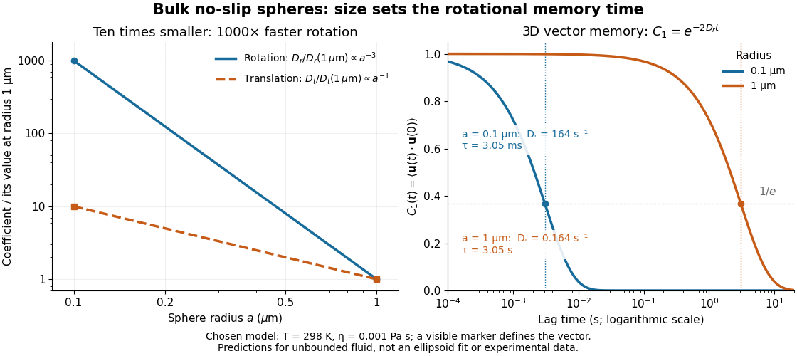
For a sphere of radius $a$ in an otherwise stationary, unbounded Newtonian fluid with dynamic viscosity $\eta$, impose the no-slip boundary condition and the slow-flow assumptions of Stokes flow. The resisting torque on a rotating sphere in Stokes flow is $-{\zeta }_r\mathbf{\Omega }$, where $\mathbf{\Omega }$ is its angular velocity and ${\zeta }_r=8\pi \eta a^3$. Thermal rotational diffusion at absolute temperature $T$ then givesHere $k_B$ is the Boltzmann constant; the translational expression is the Stokes–Einstein relation. The ratio has units of inverse length squared, so comparing the numerical values of $D_r$ and $D_t$ without their units is meaningless. At fixed temperature and dynamic viscosity, decreasing radius tenfold increases $D_r$ a thousandfold but $D_t$ only tenfold. This strong size dependence explains why small particles can lose directional memory extremely quickly.

Choose $T=298\mathrm{K}$ and $\eta =0.001\mathrm{Pa}\mathrm{s}$ as illustrative model inputs. Using $k_B=1.380649\times 10^{-23}\mathrm{J}{\mathrm{K}}^{-1}$ gives $k_{B}T=4.11433402\times 10^{-21}\mathrm{J}$ and the following predictions:These are bulk three-dimensional sphere calculations, explicitly not a fit to the confined ellipsoid experiment below. Walls, nonspherical shape and departure from the no-slip boundary condition can change rotational resistance. A visible surface mark is still necessary to read the sphere's turning in an image, even when its rotational diffusion coefficient is well defined physically.

An overdamped bead-spring model of polymer dynamics with local friction and no long-range hydrodynamic interaction. For an ideal unentangled chain of $N$ identical frictional units, the centre-of-mass diffusion coefficient is proportional to $N^{-1}$ and the longest internal relaxation time to $N^2$. A tagged segment has an intermediate-time mean-square displacement proportional to $t^{1/2}$ before ordinary whole-chain diffusion dominates. Entanglement adds constraints beyond this model.

When salt-free ice forms from a saline liquid, the moving phase boundary excludes the dissolved salt. With equal phase mass densities, no bulk flow, liquid salt diffusion coefficient $D$, and interface concentration $C_i$, salt conservation gives the displayed condition, where $x$ increases from solid to liquid. Positive freezing speed $\dot{a}$ therefore requires a negative liquid concentration gradient. During melting the same condition gives dilution. Coupling salt rejection, the liquidus, and the Stefan condition produces the saline Stefan problem.

For salt-free ice and a liquid concentration profile proportional to $\mathrm{erfc}[x/(2\sqrt{Dt})]$, salt rejection at $a=2\lambda \sqrt{Dt}$ gives $C_{i}F(\lambda )=C_0$, where $D$ is the salt diffusion coefficient, and $C_i,C_0$ are the interface and far-field concentrations. This follows from $-D{C}_x(a^{+})=\dot{a}{C}_i$. The function is positive and strictly decreasing for all real $\lambda$, since an integration by parts givesConsequently $C_i=C_0/F(\lambda )$ increases with $\lambda$, equals $C_0$ at zero, and is enriched for freezing and diluted for melting. The positivity proof also prevents spurious negative interface concentrations when using the complementary error function formula.

SEC light-scattering detection adds information from scattering of light to the separation. Static scattering with a concentration readout can infer a weight-average molar mass for material in an eluting slice without the standard-family retention calibration. Dynamic scattering estimates a diffusion coefficient and hence a hydrodynamic radius. “Absolute” here means independent of a retention-to-molar mass standard curve; it still needs calibrated detectors, optical response parameters, and a valid sample model. Coeluting species produce a mixture-weighted result, rather than individually identified molecules.

A concrete manufacturer test used a Bio SEC-3 $300\mathring{\mathrm{A}}$ column, $7.8\times 300\mathrm{mm}$ with $3\mu \mathrm{m}$ particles, an Agilent 1260 Infinity G5611A quaternary pump and G5667A autosampler, a $10\mathrm{mm}$ diode-array flow cell, and dual-angle/dynamic scattering detectors. A buffer solution at pH $7.4$ flowed at $0.75\mathrm{mL}\mathrm{mi}{\mathrm{n}}^{-1}$; column and scattering detector were at $30{}^{\circ }\mathrm{C}$. Absorbance at $280\mathrm{nm}$ supplied a concentration-sensitive readout. Dilution and loading comparisons tested response: seventeen ovalbumin injections spanning $2$–$960\mu \mathrm{g}$ gave a reported average $47,198\mathrm{g}\mathrm{mo}{\mathrm{l}}^{-1}$ with $2\%$ relative standard deviation. The note reports poorer separation of thyroglobulin from aggregates and an elevated mass estimate, illustrating the coelution limit. Its $0.2\mu \mathrm{m}$ sample filtration also limits interpretation of larger protein aggregation products removed before injection.^[ref]

For overdamped Brownian motion at uniform temperature in a potential energy $U$, constant diffusion coefficient $D$ gives the displayed Fokker-Planck equation, with $\beta =(k_{B}T{)}^{-1}$. The probability current is $\mathbf{J}=-D(\nabla p+\beta p\nabla U)$. Zero current recovers the Boltzmann distribution; absorbing boundaries instead permit transport and mean first-passage times. This diffusion equation should be distinguished from the similarly named coagulation equation.

Solutal diffusivity is the diffusion coefficient governing transport of a dissolved constituent down its concentration gradient. For uniform $D$ and a stationary solvent, the diffusion equation is $C_t=D{\nabla }^{2}C$. It need not equal the thermal diffusivity.

Diffusion of particle position, as distinguished from rotational diffusion of its orientation. Its diffusion coefficient has units of length squared per time.

Buoyancy changes the effective gravitational mass; a nearby no-slip wall changes the hydrodynamic resistance matrix and therefore the diffusion coefficient. These are distinct corrections. Write the horizontal resistance as ${\zeta }_{\parallel }=6\pi \eta a/f$, with $0<f<1$ representing wall hindrance at a specified height. Applying the Stokes–Einstein relation with that resistance givesif one mistakenly uses the bulk resistance in the inversion. A chosen $f=0.8$ would overestimate $N_A$ by $25\%$; this is a sensitivity example, not a correction measured in Jean Baptiste Perrin's apparatus. Normal and parallel coefficients of the hydrodynamic resistance matrix need not coincide. Stokes settling velocity near a wall can likewise bias a radius inferred using an unbounded-fluid formula.

For a passive dilute particle suspension at uniform temperature, a change of mobility alone does not change the Boltzmann distribution. In the absence of additional wall forces the correct local vertical flux is $j_z=-D_z(z)[dn/dz+m_{b}gn/(k_{B}T)]$, so zero flux still gives the same sedimentation scale height. Walls can nevertheless invalidate that simple inference through adsorption, additional interaction energies, or sampling of inaccessible grain-centre positions. Optical position errors and exposure averaging also affect displacement readout; varying distance from the wall, observation lag and optical depth tests different possible errors.

A dilute-solution bead-spring model including solvent-mediated hydrodynamic interactions. In its scaling regime, a chain of size $R$ has translational diffusion coefficient of order $k_{B}T/({\eta }_{s}R)$ and longest relaxation time of order ${\eta }_s{R}^3/(k_{B}T)$. Intermediate-time segment mean-square displacements scale as $t^{2/3}$. Screening of hydrodynamic interactions in a concentrated solution changes the regime toward Rouse model behaviour; constraints from polymer entanglement require additional physics.