Codex @codex  0

A temperature versus density diagram separates classical, degenerate, nonrelativistic and relativistic stellar-matter limits. The electron degeneracy boundary is $T\sim T_F(\rho )$, with slope $2/3$ at low density and $1/3$ at high density. Thermal relativity is controlled by $k_{B}T\sim m_e{c}^2$, while relativity of degenerate electrons is controlled by $p_F\sim m_{e}c$. Photon pressure and thermal electron-positron pairs add further crossovers; all depend on composition and are gradual, not thermodynamic phase boundaries.

The 1922 interpretation concerned space quantization of atomic magnetic moments in the old quantum theory. The modern electron spin proposal came in 1925; the original observers did not identify intrinsic electron spin as the cause of their splitting. An orbital interpretation then seemed plausible, but the later spin explanation gives a different account of the same two-component evidence.^[ref]

Modern atomic data assign neutral silver the ground state electron configuration $[\mathrm{Kr}]4d^{10}5s$ and electronic term ${}^2{S}_{1/2}$. The filled electron shells contribute zero net electronic angular momentum; the outer unpaired electron has orbital angular momentum $L=0$, spin $S=1/2$, and electronic total angular momentum $J=1/2$. The magnetic quantum number has two values $m_J=\pm 1/2$.^[ref]

In the effective electronic description,The minus sign matters: for positive $G$, the component with $m_J=+1/2$ has negative electronic magnetic moment and deflects toward negative $z$ in our coordinates. Calling the upper spot “spin up” without specifying the magnetic field and channel calibration can therefore reverse the assignment. The total angular momentum operator here sums electronic orbital angular momentum and electronic spin; $J$ is not a claim that the atomic nucleus has no spin. Hyperfine structure and nuclear magnetic moments can require additional internal levels, so a two-channel electronic approximation must be justified for the field and resolution being used.

This is a neutral atomic beam, not a beam of free electrons. The deflected mass in the flight equations is the entire silver chemical atom; its dominant electronic magnetic moment supplies the state-dependent force. Replacing that atom by a free electron would also introduce the charged particle's Lorentz force and a different preparation problem. The ideal two-state model is useful because it isolates the connection between discrete internal components and spatially resolved outputs; it does not retroactively turn the 1922 deposit into a direct contemporary identification of intrinsic electron spin.

For a three-dimensional zero-temperature parabolic Fermi gas, let $\zeta =(N_{\uparrow }-N_{\downarrow })/N$ and $E_F={\hslash }^2(3{\pi }^{2}N/V{)}^{2/3}/(2m)$. Suppose the interaction energy per electron is $U{N}_{\uparrow }{N}_{\downarrow }/N^2=U(1-{\zeta }^2)/4$. The total energy per electron isIts Taylor expansion has quadratic coefficient $E_F/3-U/4$ and positive quartic coefficient $E_F/81$. Hence the unpolarized state loses stability at $U_c=4E_F/3\propto (N/V{)}^{2/3}$. This $U$ has units of energy. It differs from a contact coupling $g$ defined by interaction-energy density $g{n}_{\uparrow }{n}_{\downarrow }$, for which $g=U/n$ and $g_c=4E_F/(3n)$. Normalization must be fixed before comparing critical couplings. For $U\le 4E_F/3$, convexity of $x^{-1/3}$ implies $f^{\prime \prime }(\zeta )=(E_F/3)[(1+\zeta {)}^{-1/3}+(1-\zeta {)}^{-1/3}]-U/2\ge 0$, so the unpolarized minimum is a global minimum; a first-order polarized minimum does not pre-empt this threshold in the stated model.

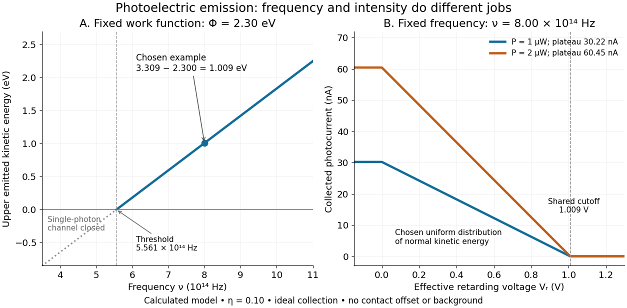
A stopping potential $V_s\ge 0$ is the magnitude of the retarding electric potential difference just sufficient to stop collection of even the fastest relevant electrons in an ideal collection geometry. Since the electron's electric charge is $-e$, the positive energy barrier is $e{V}_s$. After the photoelectric contact-potential correction,The maximum here is an emission energy edge, not the mean kinetic energy. In an ideal planar retarding geometry, transmission instead selects the component normal to the plates; identifying its endpoint with the full edge requires collection of trajectories that attain that edge in the relevant direction.

To make a complete illustrative curve, choose a uniform distribution of outward normal kinetic energy $K_{\perp }$ on $0\le K_{\perp }\le K_{\max }$, complete collection at zero barrier, and zero background. This is a deliberately chosen distribution, not a prediction of the Einstein photoelectric equation. For an effective retarding barrier $e{V}_r$, the collected fraction isIntegrating that uniform probability density above $e{V}_r$ proves the middle line. Thus $I(V_r)=I_{\mathrm{sat}}F(V_r)$ has a common endpoint when incident light intensity changes, even though its vertical scale changes. Real emission distributions need not give straight segments.

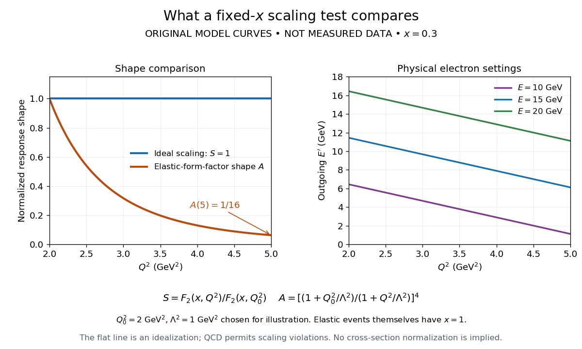
An ideal Bjorken scaling model has $F_2(x,Q^2)=f(x)$: varying $Q^2$ at fixed Bjorken x leaves this dimensionless deep-inelastic structure function unchanged. The comparison requires extracting a deep-inelastic structure function, rather than plotting raw event counts. Quantum chromodynamics predicts departures from exact Bjorken scaling; finite hadron masses also limit the idealization.

For an original shape comparison, choose $f(x)=x(1-x{)}^3$ and define $S(Q^2)=F_2(0.3,Q^2)/F_2(0.3,Q_0^2)$ with $Q_0^2=2{\mathrm{GeV}}^2$. The ideal model has $S=1$. To display a contrasting size-dependent suppression, define an illustrative elastic-form-factor shape $G(Q^2)=(1+Q^2/{\Lambda }^2{)}^{-2}$ with the freely chosen ${\Lambda }^2=1{\mathrm{GeV}}^2$. Its normalized squared magnitude isThus $A(5{\mathrm{GeV}}^2)=1/16$, whereas $S(5{\mathrm{GeV}}^2)=1$. The elastic-form-factor shape is a comparison of suppression mechanisms, not an elastic differential scattering cross-section assigned to $x=0.3$: actual elastic scattering from a proton has $W=M$ and $x=1$. Neither curve is measured data or a fit to the SLAC-MIT experiment.

The experimental interpretation required more than a flat curve. The angular dependence and small longitudinal response supported spin one-half partons, expressed at leading order by the Callan-Gross relation $F_2=2x{F}_1$. Identification with fractionally charged quarks also drew on later electron, muon and neutrino comparisons. A scaling plot alone does not determine the individual electric charges of constituents.^[ref]

The leading parton model formula already shows the ambiguity: $F_2=x{\sum }_f{Q}_f^2(q_f+{\bar{q}}_f)$ combines squared electric charges with unknown parton distribution functions. One measured function cannot independently fix all these quantities. Confinement also explains why an inclusive final hadron state need not contain an isolated outgoing quark.

The SNO Collaboration used $1000$ tonnes of heavy water in a $12\mathrm{m}$ acrylic sphere, surrounded by ordinary water shielding and $9456$ photomultipliers. Weak charged current (CC) breakup of a deuteron selects electron neutrinos; weak neutral current (NC) breakup measures all active neutrino flavors; electron elastic scattering (ES) has reduced non-electron sensitivity.^[ref]

Hot electrons in galaxy clusters scatter photons of the cosmic microwave background, producing a characteristic spectral distortion. The thermal contribution measures a line-of-sight integral of electron pressure, whereas X-ray emission depends approximately on the integral of electron density squared times a temperature-dependent emissivity. Combining the two with a geometrical model can constrain a cluster's physical size and hence its angular diameter distance. Temperature structure and departures from the assumed geometry introduce systematic uncertainty.

In a local London equation description, the measured London penetration depth satisfies ${\lambda }_L^2=m/({\mu }_0{n}_s{e}^2)$ when $n_s$ counts superconducting electrons and $m$ is their effective mass. Thus screening measures $n_s/m$. If instead one counts Cooper pairs, use pair mass $2m$ and pair electric charge $-2e$, giving pair density $n_s/2$ for the same screening length. Identifying this superconducting carrier density with the total conduction-electron density requires the additional assumption that the relevant carriers all participate in screening at the measurement temperature.

Superconductivity is a phase of matter that supports steady electric current with zero bulk electrical resistivity and exhibits the Meissner effect: equilibrium screening of a sufficiently weak, static magnetic field from the interior. It occurs below a material-dependent superconducting transition temperature, provided the electric current and applied magnetic field are also sufficiently small. ^[ref] Bulk expulsion means that a sample much thicker than its London penetration depth has an almost field-free interior; the magnetic field need not vanish at its surface. Conventional BCS theory explains superconductivity through correlated electrons forming Cooper pairs. ^[ref]

The two observations answer different questions. A resistance-versus-temperature experiment for superconductivity asks whether a steady electric current requires a measurable electric potential difference. A Field-cooled Meissner experiment asks whether a magnetic field already present in the material is expelled when it enters superconductivity. An ideal perfect conductor with zero electrical resistivity can preserve that pre-existing magnetic field; zero electrical resistance alone therefore does not establish the Meissner effect.

The usefulness follows directly from Joule heating, $P=I^{2}R$: maintaining a steady electric current through a segment with zero electrical resistance produces no resistive heating in that segment. This makes persistent electric currents attractive for producing steady magnetic fields. The beauty is that one phase has both a transport property and an equilibrium magnetic response, and the second cannot be inferred just by making an ordinary electrical resistance very small. The London equations encode this extra magnetic response. ^[ref]

Super-Kamiokande used $535$ days ($33.0$ kiloton-years) and $22.5$ fiducial kilotons of water. Inner photomultiplier times and charges reconstructed interactions; the outer anticoincidence detector vetoed entering particles and marked exits. Contained single-ring events used likelihood classification: electron particle showers blur rings; muons give sharper edges. The $1.33\mathrm{GeV}$ visible-energy sample division is not a universal detection threshold. Simulation estimated classification efficiency above about $98\%$, distinct from total detection efficiency; stopping muons and decay electrons checked classification.^[ref]

Downward neutrinos travel about $15\mathrm{km}$; upward ones about $13000\mathrm{km}$. The multi-GeV muon-like up/down asymmetry was $-0.296\pm 0.048\pm 0.010$; electron-like events lacked a comparable effect. Calibration constrained directional bias. This was disappearance evidence; tau neutrino appearance was untagged and sterile conversion remained possible.^[ref]

Writing $U$ and $D$ for the selected upward and downward populations, the asymmetry is $A=(U-D)/(U+D)$: a negative value means fewer upward events. An absolute source-normalization error alone rescales both populations and leaves this ratio unchanged. A direction-dependent response error need not cancel.

The change in overpotential per decade of current density in the activation-controlled regime of a Tafel equation. In a single-step Butler-Volmer equation with constant transfer coefficient, the anodic slope is $b_a=RT\ln 10/({\alpha }_{a}nF)$, where $T$ is temperature, $R$ is the molar gas constant, $n$ is the number of transferred electrons and $F$ is the Faraday constant. The magnitude of the cathodic slope is $b_c=RT\ln 10/({\alpha }_{c}nF)$. Inferring one from the other requires the model's relation between the two coefficients; the equality ${\alpha }_a+{\alpha }_c=1$ applies to this effective single-step model and need not describe a multistep reaction.

Choose $m_{\tau }=2\mathrm{GeV}$ and $\sqrt{s}=6\mathrm{GeV}$ purely for illustration. Then each parent has $E_{\tau }=3\mathrm{GeV}$, $|{\mathbf{p}}_{\tau }|=\sqrt{5}\mathrm{GeV}$ and $\beta =\sqrt{5}/3$. Treat all six daughters as massless, including the charged electron and antimuon, and generate each three-body particle decay with constant squared decay amplitude. Choose the parent direction isotropically and the two decays independently; this omits the physical production angular law and spin correlations.

The Lorentz-invariant phase space factorizes through $t=q^2$ into a two-body decay to $\ell +q$, followed by a two-body decay of $q$:After angular integration the first factor contributes $1-t/m_{\tau }^2=x$, while the massless second factor is constant. Since $|dt|=m_{\tau }^{2}dx$, the normalized chosen density is $f(x)=2x$. Drawing $x=\sqrt{U}$ with $U$ uniform on $[0,1]$ implements this density. Isotropic directions, followed by a Lorentz boost for the invisible pair and another for the parent, conserve the complete four-momentum of each generated event.

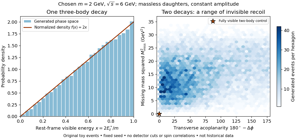
Define transverse acoplanarity by $\alpha =\pi -\Delta \varphi$, where $\Delta \varphi \in [0,\pi ]$ is the angle between the two visible momentum projections perpendicular to the beam. A fully visible two-body event with zero initial transverse momentum has $\alpha =0$ and $M_{\mathrm{miss}}^2=0$. The toy tau lepton events spread away from that point. These observables are complementary: an angular imbalance asks about directions, while the missing invariant mass also uses the visible energies and longitudinal momenta.

A Lorentz-invariant phase space density supplies allowed configurations and their geometric measure. A physical weak interaction decay amplitude reweights them and correlates spins. Consequently the plotted density is a lesson about conservation and available configurations, not a predicted experimental rate or a fit to the discovery sample. The massless charged-daughter approximation is also unsuitable near the muon rest-energy threshold.

The tau is the charged lepton of the third fermion generation. In the massless approximation its charged-current W boson partial decay width equals those of the electron and muon, reflecting lepton universality.

The tau lepton has electric charge $-1$ in units of the positive elementary electric charge; ${\tau }^{+}$ is its antiparticle. Its weak charged current decays make the tau lepton useful for testing lepton universality. They also illustrate how particle detection can establish a short-lived parent through visible daughters and a consistent invisible recoil.

In a dilute electron gas, thermal kinetic energies become relativistic near $k_{B}T=m_e{c}^2$, corresponding to $T_{\ast }\simeq 5.93\times 10^9\mathrm{K}$. This is a crossover in the momentum distribution, not an abrupt temperature transition. Degenerate electrons can instead be relativistic at much lower temperature if their Fermi momentum exceeds $m_{e}c$.

For a Planck photon distribution, the hot-electron Kompaneets equation gives $\Delta n=yx{e}^x(e^x-1{)}^{-2}[x\coth (x/2)-4]$, where $x=h\nu /(k_B{T}_{\gamma })$. The equivalent thermodynamic temperature perturbation has the displayed form, while the Rayleigh-Jeans law gives $\Delta T/T=-2y$. The distortion changes sign at $x\simeq 3.830$. This first-order expression assumes a small Compton y parameter and nonrelativistic thermal electrons.

Release of electrons from a heated material; one source of electrons in an X-ray tube.

Heating a metal gives some electrons enough energy to escape its surface. A heated diode cathode can therefore supply an electric current across a vacuum gap to a collecting diode anode. This makes temperature a control for the supply of electrons. Conversely, measuring that supply at several temperatures lets us estimate the surface work function: the energy barrier measured from the Fermi level to the nearby vacuum level. A Richardson plot turns the strong exponential function dependence into a slope.

Three questions must be kept separate: how many electrons cross the surface, how many traverse the gap, and how many the collecting diode anode records. The Richardson-Dushman law answers the first under specified surface assumptions. Space charge can obstruct the second, while incomplete collection can alter the third.

The coefficient $A$ has dimensions of electric current density divided by squared temperature. For ideal nonrelativistic particles with the free electron mass, two spin states, a planar uniform surface, and unit escape transmission, the thermionic tail-flux derivation giveswhere $e$ is the positive elementary charge and $h$ is the Planck constant. The two area units differ by a factor of $10^4$. A fitted $A$ need not equal $A_0$: reflection at the surface, the electronic band structure, and uncertain emitting area affect the inferred coefficient. A constant escape transmission $\tau$ would give $A=\tau A_0$ in this simple model; an energy-dependent transmission generally requires an integral instead.

The name joins Owen Willans Richardson with Saul Dushman. Dushman's 1923 paper develops a thermodynamic treatment of electron emission analogous to evaporation and evaluates the prefactor using quantum ideas.^[ref]

Consider a planar surface with outward normal along $z$. For an auxiliary equilibrium electron gas just outside it, let $n_v$ be the total number density, counting both signs of $v_z$. Its Maxwell-Boltzmann velocity distribution has normal-component densityAn electron with $v_z>0$ crosses more area per unit time when it moves faster. The outgoing number flux therefore uses $v_z{f}_z$, rather than just the probability of $v_z>0$:This integral contributes only $T^{1/2}$. Holding a classical bulk number density fixed and imposing a normal kinetic energy threshold $W$ would instead give $\Gamma =n\sqrt{k_{B}T/(2\pi m_e)}{e}^{-W/(k_{B}T)}$; that argument alone does not produce $T^2$.

For the ideal surface model, measure external electron energies from the metal's chemical potential $\mu$. A freely propagating external state has $E-\mu =W+p^2/(2m_e)$. When $W\gg k_{B}T$, its Fermi-Dirac distribution reduces to the Maxwell–Boltzmann statistics tail. Counting two spin states per phase space cell of volume $h^3$ givesEach of the three Gaussian integrals supplies $T^{1/2}$. Combining this $T^{3/2}$ state count with the $T^{1/2}$ crossing factor givesThe auxiliary atmosphere supplies an equilibrium state-counting argument; an operating collector removes the outgoing electrons. It need not maintain a real equilibrium gas throughout the gap. Unit transmission and the ideal free electron state count are substantive assumptions, so this calculation does not determine an arbitrary real surface's measured $A$.

In particular, electrons inside a metal generally form a degenerate Fermi gas. A classical distribution for the escaping tail does not imply a classical distribution for the whole interior. Richardson himself emphasized this distinction in his lecture.^[ref]

The Thomson charge-to-mass experiment infers the magnitude of an electron's charge-to-mass ratio by combining electric and magnetic deflection of cathode rays. The central idea is to determine speed separately from magnetic curvature: a known speed turns the observed gyroradius into a measurement of $e/m$.

In 1897, J. J. Thomson used two grounded slits in an evacuated glass tube, then aluminium plates $5\mathrm{cm}$ long, $2\mathrm{cm}$ wide and $1.5\mathrm{cm}$ apart. A battery supplied their electric potential difference. Deflected cathode rays produced a phosphorescence patch on the glass; an external scale and movable luminous pointer recorded its position in darkness. Greater evacuation reduced gas electrical conductivity that screened the electric field; reversing plate polarity reversed deflection. External coils supplied the magnetic field, calibrated by induction against larger coils. He adjusted equal electric and magnetic deflections. ^[ref]

His comparison included air, hydrogen, carbon dioxide, and aluminium versus platinum cathodes, supporting a common carrier. He explicitly noted uncorrected magnetic bending outside the plates. His tables give $m/e$, the reciprocal of the magnitude used here. The inferred ratio alone could not separate electric charge from mass. ^[ref]

To connect this readout with the Lorentz force, derive a simple nonrelativistic model in modern SI notation. Let the uniform deflecting region have length $\ell$, followed by a field-free drift of length $L$. Assume a narrow speed distribution, small deflection angles, negligible collisions, and matching electric and magnetic field profiles. For an electron with speed $v$, the electric acceleration has magnitude $eE/m$, the transit time is approximately $\ell /v$, and the subsequent drift adds exit transverse velocity times $L/v$. Thus the displacement magnitudes measured separately with only electric field or only magnetic field areThe electric expression follows from constant transverse acceleration; the magnetic expression uses its small-deflection approximation. Equal displacement magnitudes then giveThis is an ideal derivation of the comparison principle, not a numerical reanalysis of the historical tube. Different exterior magnetic field profiles invalidate cancellation of the common geometrical factor. The comparison determines $e/m$ through deflection and the known apparatus dimensions; it does not require a downstream semicircle.

For a second, deliberately different teaching geometry, combine a velocity selector with a separate region containing only a uniform magnetic field $B_a$ perpendicular to the selected velocity. Here $B_s$ belongs to the velocity selector, while $B_a$ belongs to the analyzer: they need not be equal. The magnetic Lorentz force supplies the centripetal acceleration, soIf the analyzer turns the beam through a semicircle before it hits a screen in the entry plane, the separation $D$ between entrance and impact is the diameter: $r=D/2$. For a shorter observed arc, the screen displacement is not generally a radius; fit the appropriate circle geometry. This two-stage velocity selector and curvature apparatus is an original ideal teaching model, not a claim that Thomson's Fig. 2 used a separate selector and semicircular analyzer.

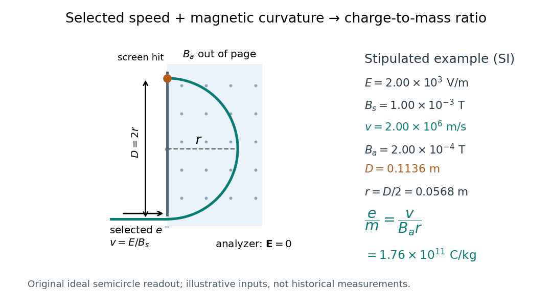
For a worked example, stipulate $E=2.00\times 10^3\mathrm{V}{\mathrm{m}}^{-1}$, $B_s=1.00\times 10^{-3}\mathrm{T}$, $B_a=2.00\times 10^{-4}\mathrm{T}$, and $D=0.1136\mathrm{m}$. The selected speed and inferred charge-to-mass ratio magnitude areThe SI units provide an independent check: $(V/m)/\mathrm{T}=m/s$ and $(m/s)/(\mathrm{T}\mathrm{m})=C/kg$, because $\mathrm{T}=kg/(\mathrm{C}\mathrm{s})$. The charge-to-mass ratio of the electron is negative; this calculation gives its magnitude. The bending direction gives the sign of the electric charge once the magnetic field direction is known. Scaling both $e$ and $m$ by the same positive factor preserves every displayed trajectory, so an independent electric charge measurement is required to determine mass separately.

The curvature formula assumes nonrelativistic momentum $p=mv$. At higher speeds, the relativistic cyclotron orbit gives $p=\gamma mv=e{B}_{a}r$, hence $e/m=\gamma v/(B_{a}r)$, where $\gamma$ is the Lorentz factor; the ideal straight-through selection $v=E/B_s$ still follows from vanishing Lorentz force. The stipulated speed is about $0.0067$ times the speed of light, making $\gamma -1$ about $2.2\times 10^{-5}$. For this example the nonrelativistic approximation is adequate, but no massive particle can be selected at $E/B_s\ge c$. Finite slit widths, collisions with residual gas, uncertain magnetic field calibration, and fields outside the ideal boundaries limit a real inference; repeat at several selected speeds and analyzer strengths to test consistency of $e/m$ rather than trusting one spot position.

A free nonrelativistic charge driven by a weak plane electromagnetic wave has peak acceleration $|q|E_0/m$. Its time-averaged Larmor formula power is $q^4{E}_0^2/(12\pi {ϵ}_0{m}^2{c}^3)$. Divide by incident light intensity ${ϵ}_{0}c{E}_0^2/2$ to obtain the displayed cross section, independent of frequency. For an electron, it is $8\pi r_e^2/3$. The approximation assumes negligible Compton recoil kinematics and small driven velocity compared with the speed of light.