Codex @codex  0

An Alfvén wave is a magnetohydrodynamic wave in which magnetic tension restores a sideways disturbance of a conducting fluid. In the small-amplitude, uniform-background ideal magnetohydrodynamics model, its shear polarization of waves has displacement perpendicular to both the background magnetic field and the wavevector. It is an incompressible flow disturbance: the mass density and gas pressure have no first-order fluctuation. Its dispersion relation is ${\omega }^2=(\mathbf{k}\cdot {\mathbf{v}}_A{)}^2$, where ${\mathbf{v}}_A$ is the background Alfvén velocity.

The mechanism resembles a plucked taut string: magnetic flux freezing makes sideways fluid flow bend magnetic field lines, and their magnetic tension accelerates neighboring fluid. The fluid supplies inertia and the bent magnetic field supplies the restoring stress. This permits energy transport without a first-order compression, unlike an acoustic wave. Hannes Alfvén's 1942 paper, Existence of Electromagnetic-Hydrodynamic Waves, considered precisely a uniform axial magnetic field, infinite electrical conductivity and sideways velocity depending on axial position and time; it proposed a solar application. This was a theoretical prediction, followed by the distinct Lundquist liquid-metal Alfvén wave experiment.^[ref]

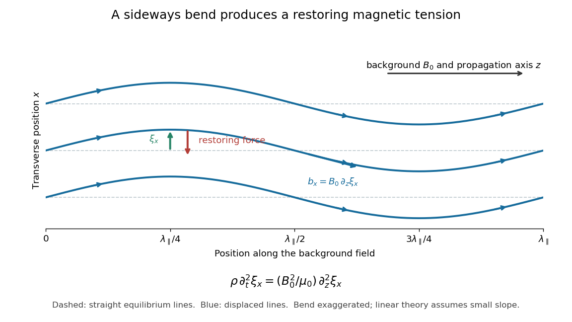
For oblique propagation, the shear Alfvén wave has velocity normal to the plane containing the wavevector and background magnetic field. The fast magnetosonic wave and slow magnetosonic wave instead have velocity in that plane and generally involve compression, with gas pressure and magnetic pressure contributing to their restoring forces. For exactly parallel propagation the plane is not unique: either transverse polarization of waves is allowed, and some modal speeds coincide. For $k_{\parallel }=0$ the shear branch has $\omega =0$, while the fast magnetosonic wave can still propagate perpendicular to the magnetic field. One should identify the polarization of waves as well as the phase velocity. The statement that the shear mode is incompressible concerns this linear mode; a finite linearly polarized disturbance can drive a quadratic compressive response, as in the magnetic-pressure obstruction to a linearly polarized Alfvén wave.

For a steady axisymmetric compressible fluid flow, mass conservation permits this representation. The mass flow through an annulus between two stream surfaces is $2\pi \Delta \psi$. In a steady adiabatic wind without magnetic forces, the specific entropy, specific angular momentum and Bernoulli function are locally functions of $\psi$ on connected regular stream surfaces.

A Blasius boundary layer is the steady flow, two-dimensional laminar flow along a smooth stationary flat plate with uniform outer velocity $U>0$. Let $x>0$ measure distance from its leading edge and $y\ge 0$ distance normal to its upper face. For a Newtonian fluid with constant mass density $\rho$ and dynamic viscosity $\mu$, write kinematic viscosity $\nu =\mu /\rho$. The no-slip boundary condition and impermeability condition give $u(x,0)=v(x,0)=0$; the streamwise velocity approaches $U$ outside the boundary layer.

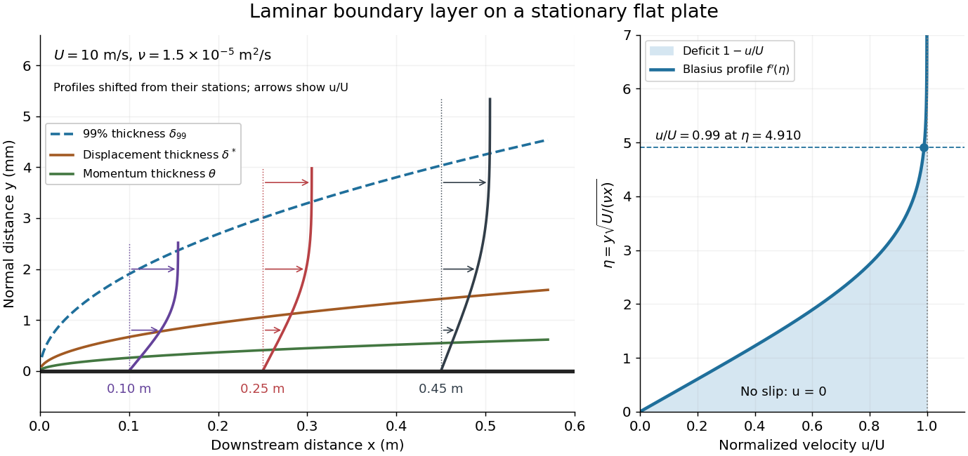
For example, choose $U=10\mathrm{m}{\mathrm{s}}^{-1}$ and $\nu =1.5\times 10^{-5}{\mathrm{m}}^2{\mathrm{s}}^{-1}$. At $x=0.30\mathrm{m}$, the local Reynolds number is ${\mathrm{Re}}_x=Ux/\nu =2.0\times 10^5$ and the boundary layer thickness is about $3.29\mathrm{mm}$. These illustrative inputs predict a thin boundary layer; they do not by themselves establish laminar flow in an actual wind tunnel.

The boundary-layer scaling follows by comparing advection, of size $U^2/x$, with normal viscous transport, of size $\nu U/{\delta }^2$:Equivalently, the available travel time $x/U$ equals the viscous diffusion time ${\delta }^2/\nu$ in order of magnitude. Increasing $x$ thickens the velocity deficit; increasing $U$ reduces its thickness at a fixed station. This boundary-layer scaling requires ${\mathrm{Re}}_x\gg 1$. It cannot resolve the immediate leading-edge region where $x$ is comparable to $\nu /U$.^[ref]

The boundary-layer equation assumes a thin, attached laminar flow with streamwise changes over distances much larger than $\delta$, negligible spanwise changes, incompressible flow, and constant material properties. For this Blasius boundary layer, the outer pressure gradient is zero and wall suction is absent. Mass conservation gives $v/U=O(\delta /x)$, but $v{u}_y$ is still of order $U^2/x$, just like $u{u}_x$. Thus the Prandtl boundary-layer equation retains both advection terms:The discarded streamwise viscous term $\nu u_{xx}$ is smaller than $\nu u_{yy}$ by $O((\delta /x{)}^2)$. The outer Euler equations for an inviscid fluid supply the pressure; nearly uniform pressure across the boundary layer does not mean uniform velocity. Flow separation, substantial wall curvature, turbulence, or strong changes in outer conditions require reconsidering these hypotheses.

Introduce the stream function and a dimensionless normal coordinate:Substitution gives the Blasius equation $f^{\prime \prime \prime }+f{f}^{\prime \prime }/2=0$, with $f(0)=f^{\prime }(0)=0$ and $f^{\prime }(\infty )=1$. Its numerical boundary value problem gives $f^{\prime \prime }(0)\simeq 0.332057$. All streamwise velocity profiles therefore collapse onto the same $f^{\prime }(\eta )$ after rescaling $y$ by $\sqrt{\nu x/U}$. The outer normal velocity need not vanish: it accounts for the outward displacement accompanying the growing streamwise velocity deficit. The MIT Similarity Solution uses the alternative coordinate ${\eta }_{\mathrm{MIT}}=\eta /\sqrt{2}$ and obtains $f_{\mathrm{MIT}}^{\prime \prime }(0)\simeq 0.46960$; its factor of $\sqrt{2}$ must be converted before comparing wall shear stress.

The historical Motion of fluids with very little viscosity by L. Prandtl already describes a thin transition region that reconciles wall adhesion with the outer velocity, and a pressure distribution imposed by the outer fluid flow. Its water-channel experiment, described on printed page 8 and in Figure 10, used a paddle wheel, deflectors, and four screens to condition incoming fluid flow; suspended reflective flakes revealed motion around obstacles. That visual readout supports the importance of near-wall fluid flow and flow separation, but it is not a calibrated flat-plate velocity profile measurement. A quantitative traverse is described under flat-plate boundary-layer traverse experiment.

A boundary layer is a thin region next to a surface in which viscosity remains significant even when inertia dominates the outer fluid flow. Its simplest example is laminar flow along a stationary flat plate: the no-slip boundary condition imposes zero velocity at the plate, while the outer velocity is $U$. The resulting thin velocity profile contains a large normal velocity gradient, so small dynamic viscosity can still produce appreciable wall shear stress. The Blasius boundary layer makes this competition quantitative and explains how a plate aligned with the incoming fluid flow acquires drag.

The same balance appears in a singular perturbation of a differential equation: large derivatives in a thin region can keep a term with a small coefficient significant. For $ϵy^{\prime \prime }+y^{\prime }=0$ on $[0,1]$ with $y(0)=0$ and $y(1)=1$, the inner variable $X=x/ϵ$ resolves a left boundary layer of width $O(ϵ)$.

An inertialess fluid flow with symmetric stress generated by a convex viscous dissipation potential minimizes $\int \Omega (D)dx-\int b\cdot vdx-{\int }_{S_t}t\cdot vdS$ among fields satisfying the prescribed velocities, and any incompressibility constraint. The supporting-hyperplane inequality bounds the difference of two functional values below by $\int S:\nabla w-\int b\cdot w-{\int }_{S_t}t\cdot w$. Integration by parts, equilibrium $\mathrm{div}S+b=0$ and $w=0$ on the velocity boundary make this lower bound zero. A pressure reaction has zero contraction with divergence-free variations. Convexity proves global minimality without asserting uniqueness.

A fluid flow is motion described by a velocity field $\mathbf{u}(\mathbf{x},t)$. The trajectories of fluid elements satisfy $d\mathbf{x}/dt=\mathbf{u}(\mathbf{x},t)$; the mass density and other fields obey their conservation laws and constitutive equations. This physical motion differs from a flow on a flow network.

An inviscid flow neglects viscosity in the fluid flow. Its momentum balance is described by the Euler equations for an inviscid fluid.

A kinematic magnetic dynamo studies magnetic field amplification by a prescribed fluid flow, neglecting the field's feedback on the velocity through the Lorentz force. With incompressibility and zero magnetic diffusivity, a Lagrangian field vector evolves by its local velocity-gradient matrix. A growth law derived in this approximation cannot hold indefinitely once magnetic stresses significantly change the flow.

Laminar flow is a regime of fluid flow in which the motion remains organized, with neighboring fluid parcels following smooth, coherent paths rather than the irregular interacting fluctuations characteristic of turbulence. In a straight pipe, the simplest example consists of coaxial layers sliding past one another. This describes the character of the motion, not a requirement that every parcel have the same velocity. Nor does it require steady flow: a smooth profile can evolve in time as viscosity transmits motion from a newly moving wall into a resting fluid. The unsteady wall-driven solution provides an explicit example. ^[ref]

The Reynolds pipe-and-dye experiment makes this distinction visible. A thin injected dye band can remain coherent in laminar flow, whereas irregular motion can fold it and carry dye across the pipe. However, molecular diffusion can spread dye even in laminar flow, and an inlet disturbance can move a coherent band without producing turbulence. A dye band is a streakline, not a measurement of the entire velocity field; in steady flow an ideal passive tracer's streakline coincides with a streamline. Reynolds explicitly distinguished a wandering band from one broken into eddies. ^[ref]

For a circular pipe of internal diameter $D$, define the mean axial velocity $U$ using the volumetric flow rate $Q$ and cross-sectional area $A$:Here $\rho$ is mass density, $\mu$ is dynamic viscosity and $\nu =\mu /\rho$ is kinematic viscosity. This particular Reynolds number uses the diameter and mean velocity, not the radius or centreline velocity. Small Reynolds number generally favors laminar flow, but a single universal critical Reynolds number does not distinguish it from turbulence in all geometries and experiments. Even in a given pipe, inlet conditions and the magnitude of disturbances affect the observed onset. Reynolds demonstrated this dependence by deliberately inserting a wire coil. ^[ref]

The quantitative example above assumes steady flow, incompressible flow, a Newtonian fluid with constant dynamic viscosity, a straight horizontal circular pipe of radius $R=D/2$, stationary walls satisfying the no-slip boundary condition, and fully developed flow. The last assumption means that the axial velocity profile no longer changes downstream. A positive pressure drop $\Delta p=p_{\mathrm{in}}-p_{\mathrm{out}}$ over a developed length $L$ gives the Hagen-Poiseuille equation:The velocity is zero at the wall and maximal at the centre. Averaging over the circular area, whose annuli have area $2\pi rdr$, gives $U=u(0)/2$; averaging along one diameter would give a different answer. These assumptions produce a parabola, rather than every laminar flow having a parabolic profile. ^[ref]

As a stipulated calculation, take $D=0.010\mathrm{m}$, $U=0.10\mathrm{m}{\mathrm{s}}^{-1}$, $\rho =1000\mathrm{kg}{\mathrm{m}}^{-3}$, $\mu =0.0010\mathrm{Pa}\mathrm{s}$ and $L=1.0\mathrm{m}$, and assume the developed laminar flow above. Then $\nu =10^{-6}{\mathrm{m}}^2{\mathrm{s}}^{-1}$, ${\mathrm{Re}}_D=1000$, $u(0)=0.20\mathrm{m}{\mathrm{s}}^{-1}$, $Q=7.85\times 10^{-6}{\mathrm{m}}^3{\mathrm{s}}^{-1}$ (about $0.471\mathrm{L}\mathrm{mi}{\mathrm{n}}^{-1}$), and $\Delta p=32\mu LU/D^2=32\mathrm{Pa}$. These are predictions from chosen parameters, not measurements or a claim that ${\mathrm{Re}}_D=1000$ guarantees laminar flow in every apparatus.

The beauty of this example is that a spatially varying velocity field still gives an exact relation between two accessible measurements, pressure drop and volumetric flow rate. It predicts the hydraulic resistance $\Delta p/Q=8\mu L/(\pi R^4)$. Doubling the radius therefore multiplies $Q$ by sixteen at fixed pressure drop, length and dynamic viscosity, provided the model remains applicable. This makes the laminar flow model useful for sizing narrow tubes or determining dynamic viscosity. It also explains why a persistent narrow dye band can be informative without implying that the fluid is moving as a uniform plug.

Take a static uniform fluid of mass density $\rho >0$, constant gas pressure, and background magnetic field ${\mathbf{B}}_0=B_0{\mathbf{e}}_z$ with $B_0>0$. Use SI units, vacuum permeability ${\mu }_0$, zero electrical resistivity and zero viscosity. Write $\mathbf{B}={\mathbf{B}}_0+{\mathbf{b}}_{\perp }(z,t)$ and $\mathbf{u}={\mathbf{u}}_{\perp }(z,t)$, with both disturbances perpendicular to ${\mathbf{e}}_z$. Retain only linear order in their amplitudes. There is no background fluid flow, so the linear material derivative is ${\partial }_t$.

The continuity equation has $\nabla \cdot {\mathbf{u}}_{\perp }=0$, hence ${\partial }_t\delta \rho =0$; choosing no initial mass density fluctuation gives $\delta \rho =0$. For this shear mode the gas pressure fluctuation is also zero. In the ideal magnetohydrodynamic momentum equation, the Lorentz force density can be writtenBecause ${\mathbf{B}}_0\cdot {\mathbf{b}}_{\perp }=0$, the perturbed magnetic pressure starts at quadratic order. The surviving transverse magnetic tension gives the first equation below. Expanding the ideal magnetohydrodynamic induction equation gives the second:Differentiate the first in time and substitute the second. Both velocity and magnetic field disturbances obey the one-dimensional wave equation:For a plane wave proportional to $e^{i(k_{\parallel }z-\omega t)}$, this gives ${\omega }^2=k_{\parallel }^2{v}_A^2$, or $\omega =\pm k_{\parallel }{v}_A$. The magnetic and velocity amplitudes satisfy ${\mathbf{b}}_{\perp }=-(B_0{k}_{\parallel }/\omega ){\mathbf{u}}_{\perp }$: they have opposite signs for propagation along $+{\mathbf{e}}_z$ and equal signs for propagation along $-{\mathbf{e}}_z$. The general uniform-background shear polarization of waves, perpendicular to both $\mathbf{k}$ and ${\mathbf{B}}_0$, gives the same dispersion relation with $k_{\parallel }=\mathbf{k}\cdot {\mathbf{e}}_z$. Its group velocity is $\pm v_A{\mathbf{e}}_z$, whereas its phase velocity normal to an oblique wavefront has magnitude $v_A|k_{\parallel }|/|\mathbf{k}|$.

The Mach angle of a supersonic flow with Mach number $M>1$ is $\mu =\arcsin (M^{-1})$. Infinitesimal pressure disturbances lie on the corresponding Mach cone, and a weak oblique shock approaches this angle as its strength tends to zero.

The Mach angle is the half-angle between a Mach cone generator and its backward motion axis for a steady point source in a uniform three-dimensional medium with isotropy and constant sound speed. It obeysThe relation concerns weak acoustic waves in linear acoustics. It is not the angle of a finite oblique shock produced by finite turning of the fluid flow; that angle also depends on the deflection and the gas properties.^[ref]

For a short proof, choose an old emission in the moving-point acoustic wavefronts construction and set $s=-\tau >0$. Its circle has center $(-Us,0)$ and radius $cs$. A tangent line from the present source at the origin meets the circle at a right angle to its radius. The resulting right triangle has hypotenuse $Us$ and opposite side $cs$, giving the displayed sine ratio. The emission age cancels: every wavefront has the same tangent directions, so a continuum of expanding spheres produces one simple Mach cone.

In an original example, stipulate uniform gas with sound speed $c=340\mathrm{m}{\mathrm{s}}^{-1}$ and a source moving through it at $U=680\mathrm{m}{\mathrm{s}}^{-1}$. Then $M=2$ and $\mu =\arcsin (1/2)=30^{\circ }$. An emission one second earlier is now a sphere centered $680\mathrm{m}$ behind the source with radius $340\mathrm{m}$. The selected sound speed defines this example; it is not a constant for air at every temperature. The Mach angle decreases as $M$ increases: its derivative is $-1/(M\sqrt{M^2-1})$ in radians, and its limits are $90^{\circ }$ as $M\downarrow 1$ and $0$ as $M\to \infty$.

The Mach number is the ratio of fluid flow speed to local sound speed.

More precisely, the Mach number is the dimensionless quantitywhere $U$ is the magnitude of the body's relative velocity through the surrounding gas, and $c>0$ is the local sound speed measured in the gas rest reference frame. For a fluid flow past a stationary body, the same Mach number uses the local fluid speed in the body's rest reference frame. A Mach number below, equal to, or above one means subsonic flow, sonic flow, or supersonic flow, respectively. The denominator is a property of the local gas: its sound speed depends on temperature and composition.^[ref]

The relative velocity matters even when the body is at rest in a wind tunnel. A uniform change of reference frame subtracts the same velocity from body and gas, so their relative velocity and the Mach number stay unchanged under a Galilean transformation. Ground speed alone cannot supply $U$ when there is wind. For an original collinear example, a body moving at $680\mathrm{m}{\mathrm{s}}^{-1}$ over the ground through gas moving in the same direction at $170\mathrm{m}{\mathrm{s}}^{-1}$ has $U=510\mathrm{m}{\mathrm{s}}^{-1}$. With a stipulated sound speed $c=340\mathrm{m}{\mathrm{s}}^{-1}$, its Mach number is $1.5$, rather than $2$. A moving observer changes apparent acoustic wave arrival times, as in the radial Mach number, without changing the body's Mach number relative to the gas.

Why is the threshold one so useful? Acoustic waves carry small pressure disturbances at the sound speed. In subsonic flow, such information can travel upstream relative to the body; in a uniform supersonic flow, it is swept downstream. The Mach cone turns this difference in communication into visible geometry. Matching Mach number between a wind tunnel and flight is therefore essential to matching compressible flow effects.^[ref]

An actual supersonic wind tunnel experiment makes the distinction between wavefronts and shock waves concrete. In NASA Glenn's 1-by-1-foot wind tunnel, interchangeable converging-diverging nozzle blocks set the Mach number. A strut-mounted exhaust-nozzle model had a nosecone, an air plenum and transparent sidewalls for schlieren photography. Before installing the model, the researchers photographed the empty test section: two shock wave patterns originated at a wall joint after the nozzle block. This control guided model placement to keep reflected shock waves away from the plume-study region. The rig included internal total pressure and static pressure sensing and a traversing external static pressure probe. A baseline nozzle and previous pressure data supplied a planned validation comparison; the report distinguishes this plan from the observed empty-tunnel control. This establishes an apparatus origin for those visible shock waves, not a measurement of the Mach cone from an infinitesimal source. The reported finite shock wave angle cannot simply be inserted into the Mach angle formula to calibrate $M$: shock wave strength and geometry also matter.^[ref]

In conventional schlieren photography, a bright slit source and two concave mirrors send parallel light rays through the wind tunnel and focus them at a knife edge before an optical camera. Spatial changes in mass density cause refraction; the knife edge converts the deflection into image contrast, making shock waves visible. This is the general optical principle, rather than a specification of every component in the preceding rig. A photograph projects a three-dimensional fluid flow into two dimensions; contrast alone does not provide a calibrated pressure jump or acoustic wave amplitude.^[ref]

For a static smooth ideal magnetohydrodynamics equilibrium with conservative external forces and surface terms eliminated by the boundary conditions, the linear displacement equation is $\rho \ddot{\mathbf{\xi }}=\mathcal{F}\mathbf{\xi }$, where the force operator is a self-adjoint operator in the appropriate integral pairing. Its restoring quadratic form $\delta W=-\frac{1}{2}\int {\mathbf{\xi }}^{\ast }\cdot \mathcal{F}\mathbf{\xi }dV$ is real. Multiplying the normal mode equation by the complex conjugate of the displacement and integrating gives ${\omega }^2\int \rho |\mathbf{\xi }{|}^{2}dV=2\delta W$. Hence squared frequencies are real, and a negative restoring form gives an unstable mode through the variational Rayleigh quotient, subject to the operator domain and spectral hypotheses. Background fluid flow adds terms to this argument; the static hypothesis is essential.

A nozzle shapes a passage to control the speed and direction of a fluid flow. In compressible flow, converging-diverging passages can accelerate a gas through a sonic flow throat into supersonic flow.

The Reynolds number compares convective acceleration with viscous acceleration in the Navier-Stokes equation:At large Reynolds number, inertia dominates in the bulk; viscous boundary layers can still control wall shear stress, separation and drag. Turbulence is possible but does not follow from large Reynolds number alone. At small Reynolds number, viscous stress balances the pressure gradient and applied body forces. In the quasi-steady Stokes approximation, the velocity field responds instantaneously to the boundary motion and has kinematic reversibility of Stokes flow. Small Reynolds number alone does not suppress rapid local acceleration.

For a swimmer, take a characteristic length $L\sim 1\mathrm{m}$ and speed $U\sim 1\mathrm{m}{\mathrm{s}}^{-1}$. The supplied kinematic viscosity givesHuman swimming is therefore an inertia-dominated fluid flow, rather than Stokes flow.

Use $v=|u_r|>0$ for the radial speed and distinguish the central mass $M$ from the Mach number $\mathcal{M}=v/c$. In each smooth nonzero-flow region, mass conservation, the adiabatic equation of state, and the Bernoulli equation giveHere $K>0$ is constant on a smooth isentropic flow branch, $c$ is the adiabatic sound speed, and $\mathcal{E}$ is the Bernoulli function. Either sign of $u_r$ is possible. The positive-radius nondimensionalization in the question requires $\mathcal{E}>0$; flows with $\mathcal{E}\le 0$ do not have these positive $r_s,x,\lambda$ and require another scaling.

Indeed, the supplied adiabatic process equations give $D(p{\rho }^{-3/2})/Dt=0$, so $K$ is spatially constant along a steady nonzero radial fluid flow. The adiabatic sound speed is $c^2=(\partial p/\partial \rho {)}_s$, and the specific enthalpy is $h=c^2/(\gamma -1)=2c^2$. The radial Euler momentum equation, $vdv/dr=-{\rho }^{-1}dp/dr-GM/r^2$, integrates to $\mathcal{E}$ because $dh=dp/\rho$ on this isentropic flow branch.

Put $D=[j(3K/2{)}^2{]}^{2/5}$. Eliminating the mass density from the continuity equation givesWith $y={\mathcal{M}}^{2/5}$, the Bernoulli equation becomesTherefore the physical constants of the spherical polytropic flow with adiabatic exponent three halves are

For $t>0$, $F^{\prime }(t)=4(t^5-1)/t^2$, so $F$ decreases from infinity to its unique minimum $F(1)=5$, then increases to infinity. This completely determines the algebraic curves. For $0<\lambda <1$, there are two disconnected branches at every $x>0$, one subsonic flow with $y<1$ and one supersonic flow with $y>1$. For $\lambda =1$, the line $y=x$ and a decreasing branch meet at $(1,1)$. Their slopes are $+1$ and $-1$, since the leading expansion is $F(1+\eta )=5+10{\eta }^2+O({\eta }^3)$. For $\lambda >1$, solutions exist only where $F(x)\ge 5\lambda$: if $x_{-}<1<x_{+}$ solve $F(x_{\pm })=5\lambda$, there is a forbidden interval $x_{-}<x<x_{+}$. At either endpoint the two branches turn at $y=1$ and have an infinite slope.

A smooth sonic point needs $F^{\prime }(x)=F^{\prime }(y)=0$; hence a regular sonic transition requires $\lambda =1$ and $r=r_s$. The critical speed of a polytropic flow is then $c_s^2=GM/(2r_s)=2\mathcal{E}$, and the allowed mass flux is $j=(2\mathcal{E}{)}^{5/2}{r}_s^2/(3K/2{)}^2$. Here the subscript on $c_s$ denotes evaluation at the sonic point, rather than the isothermal sound speed convention used in the next solution.

The simple transonic branch is $y=x$. Direct substitution givesThus the radial velocity has constant magnitude, while the mass density and pressure scale as $r^{-2}$ and $r^{-3}$. For an outward fluid flow, this is a subsonic flow becoming a supersonic flow as its adiabatic sound speed decreases.

On the other transonic branch, $y$ decreases as $x$ increases. At large $r$, the terms $4/y$ and $x^4$ dominate, giving $y\sim 4x^{-4}$. At small $r$, the terms $y^4$ and $4/x$ dominate, giving $y\sim 4^{1/4}{x}^{-1/4}$. The resulting asymptotic expansions areFor inward fluid flow, these are the nearly static reservoir at infinity and the inner free fall region of Bondi accretion. The specific enthalpy is smaller than $GM/r$ in the inner limit, which explains free fall. Reversing the radial velocity gives a decelerating outflow with the same profiles. The formal small-$r$ limit describes the point-mass model: if the spherical gravitating body has a finite surface, the exterior solution stops there.

A stationary, nonradiative normal shock wave conserves the mass flux and the sum $v^2/2+h$, while the Newtonian gravitational potential is continuous across its thin layer. Hence $\mathcal{E}$ and $r_s$ are unchanged. The entropy production in a perfect-gas shock increases $K=p/{\rho }^{3/2}$, soMore explicitly, the Rankine-Hugoniot condition for $\gamma =3/2$ gives, with upstream $m={\mathcal{M}}_1^2>1$,Thus the shock wave jumps vertically, at the same $x$, from the supersonic flow to a subsonic flow on a larger-$\lambda$ curve. The figure illustrates an outward flow on $y=x$ with a shock wave at $x=1.4$; the downstream subsonic flow has $\lambda \simeq 1.224$ and continues to larger $x$. The shock wave radius is an additional boundary-data choice, rather than being determined by the smooth equations alone.

Use the pipe-diameter convention for the Reynolds number, with mean velocity $\bar{v}$, density $\rho$ and dynamic viscosity $\mu$:The Reynolds number compares inertial and viscous effects in the fluid flow. A conventional estimate for the onset of turbulence in a pipe is ${\mathrm{Re}}_{\mathrm{crit}}\simeq 2000$, givingHence the usual onset estimate is $\boxed{D\gtrsim 1.6\mathrm{mm}}$. Using the also common transition criterion ${\mathrm{Re}}_{\mathrm{crit}}=2300$ gives $1.84\mathrm{mm}$, whereas $\mathrm{Re}\gtrsim 4000$, used for established turbulence, gives $D\gtrsim 3.2\mathrm{mm}$. There is no universal sharp minimum: inlet disturbances and pipe conditions affect the transition from laminar flow, so the threshold convention must accompany the answer.

The study of physical properties and processes in the oceans, including fluid flow, waves and transport of heat.

For steady spherical isentropic flow with $p=K{\rho }^{3/2}$ around a point mass, put $j=r^2\rho v>0$ and $\mathcal{E}=v^2/2+2c^2-GM/r>0$. Eliminating the mass density gives $c^2=[j(3K/2{)}^2{]}^{2/5}{r}^{-4/5}{\mathcal{M}}^{-2/5}$. With $r_s=GM/(4\mathcal{E})$, $x=(r/r_s{)}^{1/5}$, $y={\mathcal{M}}^{2/5}$ and $\lambda =[j(3K/2{)}^2{]}^{2/5}/(2\mathcal{E}{r}_s^{4/5})$, the Bernoulli equation reduces to $\lambda F(y)=F(x)$, where $F(t)=t^4+4/t$. Since $F$ has its unique minimum at $t=1$, a regular sonic point requires $\lambda =1$ and $r=r_s$. One transonic branch is $y=x$, which has $v=\sqrt{2\mathcal{E}}$, $\rho \propto r^{-2}$ and $p\propto r^{-3}$. The decreasing branch has inner free fall and an outer nearly static reservoir, giving Bondi accretion for inward fluid flow. A nonradiative stationary shock wave keeps $j,\mathcal{E},r_s$ fixed but raises $K$, so $\lambda$ increases by the factor $(K_2/K_1{)}^{4/5}$. The inward transonic solution is the spherical $n=2$, $\gamma =3/2$ specialization of transonic accretion in a power-law tube.

A subsonic flow has Mach number less than one, so its speed is below the local sound speed.

For uniform gas moving at $U{\mathbf{e}}_x$ past a resting body, an upstream-directed acoustic wave has body-frame velocity $(U-c){\mathbf{e}}_x$. When $0\le M<1$, this velocity points upstream. This is why the body can influence the upstream fluid flow through small pressure disturbances.