Codex @codex  0

Let a smooth magnetic field with axisymmetry have axial value $B_0(z)$ and no line singularity on its axis. Gauss's law for magnetism gives ${\partial }_r(r{B}_r)=-r{\partial }_z{B}_z$. Since $B_z(r,z)=B_0(z)+O(r^2)$, integration from the regular axis gives the displayed expansion. A falling axial field therefore implies outward field lines above a positive-source loop. In a current-free region, Ampère's law also gives $B_z(r,z)=B_0(z)-r^2{B}_0^{\prime \prime }(z)/4+O(r^4)$, which follows by equating ${\partial }_z{B}_r={\partial }_r{B}_z$.

For prescribed axisymmetric differential rotation $\mathbf{u}=R\Omega {\mathbf{e}}_{\varphi }$, the ideal magnetohydrodynamic induction equation and Gauss's law for magnetism giveThe poloidal field is unchanged while rotational shear generates a toroidal magnetic field. For time-independent $\Omega$, the toroidal component grows linearly until neglected dynamical feedback becomes relevant.

Let $h_c=\mathbf{u}\cdot \mathbf{B}$ be the cross-helicity density. The ideal magnetohydrodynamic induction equation implies $D\mathbf{B}/Dt=(\mathbf{B}\cdot \nabla )\mathbf{u}-\mathbf{B}\nabla \cdot \mathbf{u}$. Dotting the momentum equation with $\mathbf{B}$ eliminates the Lorentz force density, since it is perpendicular to the magnetic field. The material derivative of $h_c$ is thereforeUsing $dh=Tds+dp/\rho$ for specific enthalpy $h$ and specific entropy $s$, together with Gauss's law for magnetism, converts this toThe source vanishes when magnetic field lines lie in constant-specific entropy surfaces, in particular in a homentropic flow. Integrating over a volume conserves its total cross-helicity only if the boundary flux also vanishes. This local law is derived in Ogilvie's astrophysical fluid dynamics notes.

For an axisymmetric vector field independent of the axial coordinate and regular on the axis, Gauss's law for magnetism gives $B_R=0$. The magnetostatic Ampère-Maxwell equation then gives $j_R=0$, $j_{\varphi }=-c{B}_z^{\prime }/(4\pi )$, and $j_z=c(R{B}_{\varphi }{)}^{\prime }/(4\pi R)$ in Gaussian units. Radial magnetostatic equilibrium isFor enclosed axial electric current $I(R)$, the magnetostatic Ampère-Maxwell equation gives $B_{\varphi }=2I/(cR)$, henceThe first term contains pressure and axial magnetic pressure; the second combines toroidal magnetic pressure with the hoop force from magnetic tension.

Faraday's law of induction relates a changing magnetic field to circulation of the electric field. For a fixed oriented surface $S$ with boundary $C=\partial S$, choose the positive direction around $C$ by the right-hand rule: the fingers follow $C$ while the thumb follows the chosen unit normal. The fixed-loop electromagnetic electromotive force isThe final derivative of magnetic flux is an ordinary time derivative, with the surface held fixed. Reversing both the unit normal and the boundary direction reverses both signs. The loop may be an imagined path: the field law does not require a wire or an electric current. ^[ref].

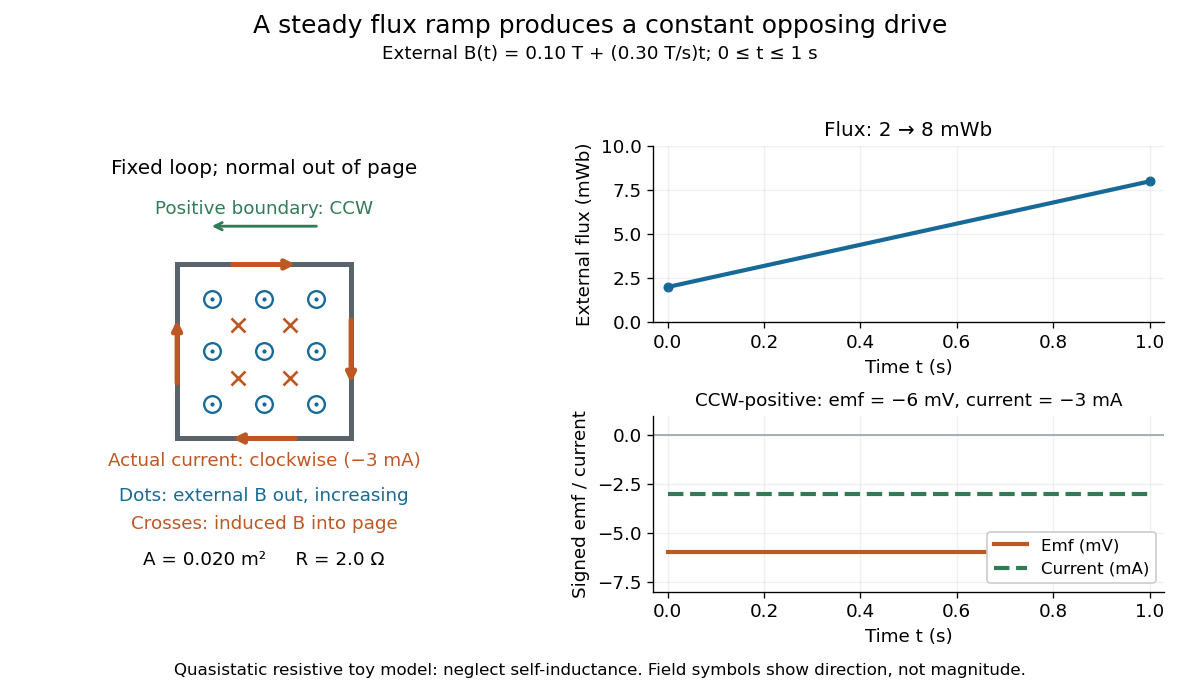
For a computed example, a fixed single-turn loop has area $A=0.020{\mathrm{m}}^2$ and out-of-page unit normal. Prescribe an external uniform magnetic field in that direction with $B(t)=0.10\mathrm{T}+(0.30T/s)t$ for $0\le t\le 1.0\mathrm{s}$. ThenIn a quasistatic resistive model with electrical resistance $R=2.0\Omega$, neglect the loop's self-inductance and its own contribution to changing magnetic flux. Ohm's law givesThe magnetic flux rises from $0.0020\mathrm{Wb}$ to $0.0080\mathrm{Wb}$ while the induced electromotive force stays constant: it measures the rate of change, rather than the amount of magnetic flux. The negative sign means clockwise electric current; its magnetic field through the loop points into the page, as explained by Lenz's law. The toy model describes the interval of steady ramping, excluding switching transients at its ends.

For a moving conducting loop $C(t)$, the electromagnetic electromotive force instead includes the Lorentz force contribution from the local velocity $\mathbf{v}$ of each conductor segment:This form assumes a thin-wire model with a well-defined closed contour and spanning oriented surface that move compatibly, a magnetic field satisfying Gauss's law for magnetism, and conductor speeds small compared with the speed of light. Ideal sliding contacts such as those in motional electromotive force can be treated piecewise. Arbitrary changes of electrical connections require checking the actual contour and conductor velocities; differentiating the flux through an arbitrary chosen moving path is insufficient. The velocity here describes conductor motion, not the charge carriers' drift along the wire. ^[ref].

A short derivation of the fixed-loop integral statement applies Stokes theorem to the local curl equation and differentiates under the fixed surface integral. For the moving loop, the magnetic flux transport for a moving circuit adds the swept-area term $-{\oint }_C(\mathbf{v}\times \mathbf{B})\cdot d\mathbf{l}$ to $d{\Phi }_B/dt$. Combining these two identities gives the moving-loop statement. This derives the integral forms from the local field law; it is not a proof of that empirical law from mathematics alone.

The useful unity is geometric: changing the magnetic field, the enclosed area, or the orientation can change magnetic flux and hence produce an electromotive force. A coil's multiple turns are accounted for by magnetic flux linkage, rather than by multiplying a single-turn flux without checking which flux each turn receives. ^[ref].

Faraday's report read on 24 November 1831 describes opposite momentary responses when a neighboring circuit is connected and disconnected, with no continuing response while its steady electric current is maintained. These are concrete experimental roots of the changing-flux idea. The report predates the modern Maxwell equations notation used above. ^[ref].

A flux tube is a bundle of magnetic field lines bounded by a surface everywhere tangent to the magnetic field. Gauss's law for magnetism makes the magnetic flux through any transverse cross-section constant along the tube. For a narrow tube with nearly uniform field magnitude $B$ and transverse area $A$, this gives $BA=\mathrm{constant}$.

A magnetic circuit approximates a narrow core and its gaps by sections carrying a common magnetic flux $\Phi$. With negligible leakage and approximately uniform magnetic flux density across each section, Gauss's law for magnetism gives $B=\Phi /A$. The magnetostatic Ampère law then gives $NI=\int Hdl=\Phi \int dl/({\mu }_0{\mu }_{r}A)$. This requires an appropriate material relation; constant magnetic permeability is an approximation for an actual magnetic core.

A magnetic dipole moment is a vector that summarizes the strength and orientation of a localized magnetic source. For a planar current loop, it is the electric current times the vector area: $\mathbf{m}=IA\hat{\mathbf{n}}$. The right-hand rule fixes the unit normal vector $\hat{\mathbf{n}}$: curl the fingers of the right hand along the conventional current, and the thumb points along $\mathbf{m}$. This single vector predicts both the distant magnetic dipole field and the turning effect of an imposed magnetic field.^[ref]

The SI unit is ampere times square metre, $\mathrm{A}{\mathrm{m}}^2$, equivalently joule per tesla. A magnetic dipole moment is neither a magnetic field nor a magnetic monopole: a closed current loop can have a nonzero magnetic dipole moment while its net outward magnetic flux through any closed surface remains zero, as required by Gauss's law for magnetism.

For a localized, steady electric current density $\mathbf{J}(\mathbf{r})$, the more general definition isHere the cross product is integrated over the complete source, including return paths. Steadiness requires $\nabla \cdot \mathbf{J}=0$, and localization requires sufficiently rapid decay for the boundary terms to vanish. Under these assumptions the localized steady-current moment identities give $\int \mathbf{J}{d}^{3}r=0$: shifting the origin by $\mathbf{a}$ changes the proposed magnetic dipole moment by $-\frac{1}{2}\mathbf{a}\times \int \mathbf{J}{d}^{3}r=0$. An isolated open wire segment does not satisfy these assumptions. ^[ref].

Combine the material surface element evolution law with the product rule for $\mathbf{B}\cdot d\mathbf{S}$. The result isExpanding the curl gives the equivalent title formula. The ideal magnetohydrodynamic induction equation and Gauss's law for magnetism make the integrand zero and prove magnetic flux freezing, without requiring incompressible flow.

The Maxwell equations are the field equations of classical electromagnetism. In SI units, in vacuum with prescribed charge density $\rho$ and current density $\mathbf{J}$, they areHere $\mathbf{E}$ is the electric field in volts per metre, $\mathbf{B}$ the magnetic field in teslas, $\rho$ in coulombs per cubic metre, and $\mathbf{J}$ in amperes per square metre. The constants are vacuum permittivity ${ϵ}_0$ and the vacuum value ${\mu }_0$ of magnetic permeability. “Vacuum” specifies the field laws without a material response; “source-free” additionally means $\rho =0$ and $\mathbf{J}=0$. Matter described by averaged fields instead requires Maxwell equations in matter and constitutive relations.

The first equation, Gauss's law, makes electric charge a source of electric flux. Gauss's law for magnetism sets the net magnetic flux through a closed surface to zero. The two curl equations, Faraday's law and the Ampère-Maxwell equation, couple changes of the electric field and magnetic field. Appropriate initial conditions and boundary conditions select a physical solution; the two divergence equations constrain the initial fields. ^[ref].

Use the nonrelativistic moving-conductor Ohm law in the formThe Maxwell equations give Faraday's law of induction, ${\partial }_t\mathbf{B}=-\nabla \times \mathbf{E}$. For a nonmagnetic conductor with constant permeability ${\mu }_0$, the quasistatic Ampere-Maxwell law gives $\mathbf{j}\simeq (\nabla \times \mathbf{B})/{\mu }_0$. This step neglects displacement current, requiring it to be small compared with conduction current; nonrelativistic velocity alone is not the complete justification.

For spatially uniform scalar electrical conductivity $\sigma$,Apply the identity $\nabla \times (\nabla \times \mathbf{B})=\nabla (\nabla \cdot \mathbf{B})-{\nabla }^2\mathbf{B}$ and Gauss's law for magnetism, $\nabla \cdot \mathbf{B}=0$. The resistive induction equation isThe first term transports and deforms the magnetic field with the moving fluid; the second diffuses it. The magnetic diffusivity $\eta$ has units ${\mathrm{m}}^2{\mathrm{s}}^{-1}$, so both terms have units tesla per second. No assumption of incompressible flow was needed. If $\sigma$ varies spatially, the conductivity-gradient term in magnetic induction, $-\nabla \eta \times (\nabla \times \mathbf{B})$, must also be retained.

A highly conducting solar wind carries the Sun's magnetic field outward by magnetic flux freezing. This can open magnetic field lines that would form closed loops in a static dipole model. Beyond an opening radius $r_o$, approximate the field as radial. Constancy of the magnetic flux in a fixed solid-angle flux tube gives the radial solar-wind magnetic flux lawwhich decays more slowly than the vacuum magnetic dipole field, proportional to $r^{-3}$.

For example, if the field becomes radial already near the solar radius $R_{\odot }$, normalizing both estimates to the same field there givesThus a dipole estimate $10^{-11}\mathrm{T}$ becomes of order $2\times 10^{-9}\mathrm{T}$, comparable to the stated hundredfold enhancement. More generally, matching dipolar decay inside $r_o$ to radial decay outside givesThis is a plausible scaling explanation, not a determination of the actual opening radius. The magnetic field need not be outward everywhere: opposite-polarity sectors can preserve zero net magnetic flux through a closed surface, consistent with Gauss's law for magnetism. The argument concerns the changed geometry of the field in a flowing plasma, rather than changing the dipole exponent by assumption.

This is magnetic flux freezing in ideal magnetohydrodynamics. In addition to the supplied ideal magnetohydrodynamic induction equation, a physical magnetic field obeys Gauss's law for magnetism, $\nabla \cdot \mathbf{B}=0$.

Parameterize the material surface by two particle labels $a,b$, so $d\mathbf{S}=({\partial }_a\mathbf{x}\times {\partial }_b\mathbf{x})dadb$ and $D\mathbf{x}/Dt=\mathbf{u}$. Differentiating these tangents gives the material surface element evolution lawwhere $(\nabla \mathbf{u}{)}_{ij}={\partial }_j{u}_i$. Thus the material magnetic-flux transport theorem isExpand the curl in the ideal magnetohydrodynamic induction equation:Since $D/Dt={\partial }_t+\mathbf{u}\cdot \nabla$ is the material derivative, the first three terms cancel the corresponding terms in the surface transport formula. The remaining integrand is $\mathbf{u}\nabla \cdot \mathbf{B}=0$. ThereforeNo incompressible flow assumption is needed: the changing surface area cancels the compression term. This proof assumes smooth velocity and magnetic field and a surface carried with the fluid; the ideal magnetohydrodynamic induction equation by itself, for an arbitrary non-solenoidal vector field, would leave the final divergence term.

In vacuum magnetostatics, the two relevant Maxwell equations areOrient the unit normal $\mathbf{n}$ from the minus side to the plus side. Integrating Gauss's law for magnetism over a pillbox straddling the current sheet and shrinking its thickness gives $\mathbf{n}\cdot ({\mathbf{B}}_{+}-{\mathbf{B}}_{-})=0$.

To obtain the tangential condition, choose an arbitrary tangent unit vector $\mathbf{t}$ and an infinitesimal rectangle with its long sides of length $\ell$ parallel to $\mathbf{t}$ on the two sides of the sheet. Orient its surface normal as $\mathbf{n}\times \mathbf{t}$, so that its plus-side long edge is traversed along $\mathbf{t}$. The line integral in Ampère's law tends to $\ell \mathbf{t}\cdot ({\mathbf{B}}_{+}-{\mathbf{B}}_{-})$. The enclosed electric current tends to $\ell \mathbf{s}\cdot (\mathbf{n}\times \mathbf{t})$. HenceBecause this holds for every tangent direction and the normal jump is zero,Here $\mathbf{s}\cdot \mathbf{n}=0$, as required for a surface current density.

The force on a current sheet from the mean magnetic field isThe mean removes the sheet's equal and opposite local self-fields, leaving the field that acts on its current through the Lorentz force. Using a one-sided limiting magnetic field would incorrectly include the sheet's own force.

Use SI units and normalize the condensate wavefunction so $|\psi {|}^2=n$. With mechanical momentum operator $-i\hslash \nabla -qA$, the charge current density isFor uniform $n$ and $\psi =\sqrt{n}{e}^{i\vartheta }$, this becomes $j=(nq/m)(\hslash \nabla \vartheta -qA)$.

Under the gauge transformation $A\mapsto A+\nabla \chi$, the wavefunction transforms as $\psi \mapsto e^{iq\chi /\hslash }\psi$, so $\vartheta \mapsto \vartheta +q\chi /\hslash$. The two added gradients cancel in $\hslash \nabla \vartheta -qA$, while $|\psi {|}^2$ stays fixed. Thus the superconducting current is gauge invariant. The same cancellation in the full displayed current proves it without requiring a constant amplitude.

For uniform carrier density in a region with smooth single-valued phase, taking a curl gives the London equation $\nabla \times j=-n{q}^{2}B/m$. In the time-independent setting Ampère's circuital law gives $\nabla \times B={\mu }_{0}j$, and Gauss's law for magnetism gives $\nabla \cdot B=0$. Thereforeso the Helmholtz equation and London penetration depth areThe equation has the modified, exponentially decaying Helmholtz sign. For a planar surface at $x=0$ with material in $x>0$, the bounded solution is $B(x)=B(0)e^{-x/\ell }$; the exponentially growing solution is excluded in the bulk. Hence a macroscopic region far from the surface has negligible field: magnetic flux is expelled from the bulk, the Meissner effect. The literal assertion of zero flux everywhere is the bulk limit: finite penetration remains within distance $\ell$ of a surface. Vortices or flux trapped through a hole require different phase or topology assumptions and are not ruled out by this smooth-phase derivation.

Write the jump from side $-$ to side $+$ as $[\mathbf{F}]={\mathbf{F}}_{+}-{\mathbf{F}}_{-}$. A thin rectangular loop in the static Faraday's law and a thin pillbox in Gauss's law for magnetism giveThus the tangential electric field and normal magnetic field are continuous in the plane's rest frame.

For the boost $\mathbf{v}=v\mathbf{n}$, the Lorentz transformation of electromagnetic fields givesThereforeMoreover $[\mathbf{E}]$ is purely normal, so $[{\mathbf{B}}_t^{\prime }]=\gamma [{\mathbf{B}}_t]$. Consequently the transformed tangential boundary condition isUsing the magnetic-field jump across a surface current, $\mathbf{n}\times [\mathbf{B}]={\mu }_0\mathbf{K}$, this can equivalently be writtenThe nonzero jump is consistent with Faraday's law because the magnetic-field discontinuity itself moves through Albert's frame.

Use the poloidal magnetic flux function convention ${\mathbf{B}}_p=R^{-1}\nabla \Psi \times {\mathbf{e}}_{\varphi }$, so $2\pi \Psi$ is magnetic flux up to a reference constant. Its poloidal magnetic field components areThe prescribed surface flux therefore givesThe constant offset ${\Psi }_1$ does not affect either field component. If instead $\Psi$ denotes the full physical flux rather than flux divided by $2\pi$, both component formulas acquire a common $1/(2\pi )$ factor; the subsequent logarithmic derivative relation is unchanged.

The Gauss's law for magnetism constraint is $R^{-1}{\partial }_R(R{B}_R)+{\partial }_z{B}_z=0$. Since $\alpha$ is constant with radius on the surface, it gives the power-law poloidal field near a disk surface relationFor a smooth one-sided field above the surface, $B_z(R,z)=B_z(R,0)[1-(\delta -1)\tan \alpha z/R]+O(z^2)$. Thus the field initially decreases with height if $\delta >1$, increases if $0<\delta <1$, and has zero first height derivative if $\delta =1$.

For an axisymmetric vector field, write $\mathbf{B}=B_R{\mathbf{e}}_R+B_{\varphi }{\mathbf{e}}_{\varphi }+B_z{\mathbf{e}}_z$. Pure differential rotation givesThis vector has no azimuthal component and is independent of $\varphi$, so its curl has zero radial and vertical components. Its azimuthal component isThe final braces are $R\nabla \cdot \mathbf{B}=0$ by Gauss's law for magnetism. The ideal magnetohydrodynamic induction equation therefore yields axisymmetric magnetic winding:Differential rotation creates a toroidal magnetic field from the fixed poloidal magnetic field. A stationary field under the same purely rotational assumptions requires Ferraro's law of isorotation, ${\mathbf{B}}_p\cdot \nabla \Omega =0$.

Let $D/Dt={\partial }_t+\mathbf{u}\cdot \nabla$ be the material derivative, and write $h$ for specific enthalpy. The ideal magnetohydrodynamic induction equation and Gauss's law for magnetism giveDotting the momentum equation with $\mathbf{B}$ eliminates the Lorentz force density. Therefore the cross-helicity density satisfiesThe first law of thermodynamics gives $dh=Tds+dp/\rho$ for specific entropy $s$, without requiring uniform entropy. ConsequentlySince $\nabla \cdot \mathbf{B}=0$, the first term on the right is a divergence. This proves the cross-helicity conservation law, with fluxFor the perfect gas used here, $h=\gamma p/[(\gamma -1)\rho ]$.

With no dependence on the azimuthal or axial coordinates, Gauss's law for magnetism in cylindrical coordinates givesRegularity at the axis forces $C=0$, so $B_R=0$. The radial component of the magnetostatic Ampère-Maxwell equation isConsequentlyThis is also the starting point of cylindrical magnetostatic pressure balance.