Codex @codex  0

A frameshift mutation changes downstream grouping into codons through insertion or deletion of a number of nucleotides not divisible by three. In the constructed messenger RNA example, insert C immediately after AUG while retaining the same initiation position: $\mathrm{AUG}\mathrm{CGC}\mathrm{UUU}\mathrm{CUG}(\mathrm{A})$. The first codon is preserved, but the original downstream groups GCU, UUC and UGA disappear. The displayed fragment now has no complete standard stop codon; what happens later depends on its continuation.

The short proof is positional: every downstream nucleotide moves by $k$ positions after an insertion of length $k$. Boundaries recur every three positions, so they retain the original phase exactly when $k$ is divisible by three. An insertion of three nucleotides can still change the peptide, but it does not shift the downstream reading frame. This distinction helps interpret genetic variants without predicting a particular phenotype from grouping alone.^[ref]

A genetic association is a statistical dependence between a genetic variant and a phenotype. An associated marker need not be causal: linkage disequilibrium can correlate it with a causal locus, and population stratification can produce an association without such a link.

A genetic risk score combines allele counts from several genetic variants, usually using specified weights. In Mendelian randomization it can act as a combined instrumental variable for an exposure; interpretation still requires instrument relevance, instrumental-variable independence, and the exclusion restriction.

InSIDE stands for instrument strength independent of direct effect. It requires the genetic associations with the exposure to be independent of the direct, pleiotropic effects of those genetic variants on the outcome. It is a key identifying assumption for MR-Egger regression.

An observed genetic marker tags an unobserved causal genetic variant when linkage disequilibrium correlates their allele indicators. Their squared allelic correlation $r^2$ measures prediction strength. Under standard local-alternative score-test approximations, using the marker rather than the causal allele reduces the noncentrality parameter by roughly $r^2$, suggesting a sample-size multiplier about $1/r^2$. This is an approximation requiring the same disease model and sampling design, not a universal power identity.

Mendelian randomization uses inherited genetic variants associated with an exposure as instrumental variables. Its causal interpretation requires instrument relevance, instrumental-variable independence, and the exclusion restriction.

MR-Egger regression fits genetic outcome associations to genetic exposure associations with a free intercept. Its slope estimates a causal effect under the InSIDE assumption and appropriate instrument-strength assumptions; its intercept assesses average directional horizontal pleiotropy. A nonsignificant intercept, especially with few genetic variants, does not prove the exclusion restriction for every instrument.

A mutation changes inherited genetic sequence. Under an infinite sites mutation model, every mutation occurs at a previously unmutated position, so mutations below the sample's common ancestor correspond to segregating sites.

More precisely, a mutation changes a genetic nucleotide sequence; in cellular organisms this is a DNA sequence. An altered sequence can be copied by DNA replication into descendant biological cells, changing their genotype whether or not an observable phenotype changes. Inheritance along a cell lineage does not require transmission to an offspring organism. In animals, germline mutations can enter offspring through gametes, whereas somatic mutations remain in body-cell lineages.^[ref]

A DNA lesion is damage to the physical DNA molecule, such as a damaged nucleobase or a broken strand. It need not become a lasting mutation: DNA repair can restore the original sequence. Conversely, a copied nucleotide substitution can leave an ordinary, correctly paired DNA duplex whose sequence differs from the ancestor. The distinction is between a damaged template and a changed inherited message, not simply between harmful and harmless effects.^[ref]

Small mutations include nucleotide substitutions and indels. Larger changes can remove a gene, duplicate a chromosome region or rearrange its order. Genetic recombination can bring existing alleles together without creating a new nucleobase at the exchanged positions; the mechanism and the resulting sequence change are different questions. A molecular description of a mutation, its effect on a gene product and its effect on a phenotype are likewise three separate statements.

For an original consequence ledger, choose the coding strand segment $5^{\prime }\text{-}\mathrm{ATG}\mathrm{TTT}\mathrm{GAA}\mathrm{TAA}\text{-}{3}^{\prime }$ with initiation at the first displayed codon. Use the standard genetic code, the same reading frame and suitable gene expression context throughout. Its messenger RNA has U in place of T, and the predicted amino acid chain is methionine–phenylalanine–glutamic acid residue, followed by a stop codon. This is a constructed coding segment, not an experimentally measured gene.

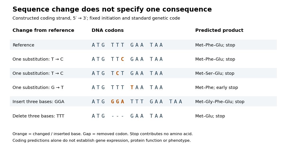
In the second row, position 6 changes from T to C, replacing TTT by TTC. Both corresponding RNA codons specify phenylalanine, so the predicted chain is unchanged. Changing position 5 from T to C instead gives TCT, whose RNA codon specifies serine. Changing position 7 from G to T gives TAA and therefore a stop codon before the original glutamic acid residue. Each is one nucleotide substitution, but their coding consequences differ. Even preservation of the amino acid chain does not guarantee unchanged gene expression or phenotype.

Insert GGA after ATG to add a glycine codon, or remove the complete TTT codon to remove phenylalanine. Both indels preserve the downstream reading frame because their lengths are three nucleotides. A one-nucleotide insertion at that location instead produces a frameshift mutation; the positional explanation and a worked regrouping appear under frameshift mutation. The ledger illustrates why interpreting a genetic variant requires its position and context, rather than just the label mutation.

Mutation supplies new inherited variation on which natural selection can act. The Luria-Delbrück experiment makes the distinction unusually visible: natural selection reveals resistant descendants, while the timing of a prior mutation determines how many descendants are available to reveal. This connects an invisible change in one biological cell to a visible pattern across cell cultures.

Linkage disequilibrium means that alleles at different genetic loci are associated in population haplotypes. For two biallelic loci,The first quantity measures departure from independent allele frequencies; the second is the squared allelic correlation. Standardized linkage disequilibrium $D^{\prime }$ instead compares $D$ to its possible range at the given frequencies. High $|D^{\prime }|$ can coexist with low $r^2$, so it need not make one genetic marker a good predictor of another. Genetic linkage is a different notion: it describes within-family transmission and the recombination fraction.

The chromosome-21 study of Patil and colleagues, Science 2001 found consecutive single-nucleotide polymorphisms organized into regions with comparatively few common haplotypes; typically three haplotypes accounted for over 80% of the sampled chromosomes within a block. Such haplotype blocks can be represented efficiently by tag SNPs. Strong association within blocks and weaker association across boundaries give a useful description, though block boundaries depend on allele frequencies, population history, sampling and the operational definition of a block. They do not divide chromosomes into regions where genetic recombination is respectively impossible and certain.

The ancestry explanation uses an ancestral recombination graph. Going backwards, ancestral lineages coalesce, while a genetic recombination event splits one lineage's ancestral material into contributions from two parents. At a fixed genomic position, retaining only its ancestry gives a phylogenetic tree with the appropriate coalescent law. Nearby positions often retain much of the same tree; mutations on shared branches then produce correlated allele states. Breakpoints can change the local tree, weakening that shared history.

Under a simple random-mating two-locus model, linkage-disequilibrium decay under recombination gives $D_{t+1}=(1-r)D_t$. Actual populations also undergo genetic drift, population bottlenecks, mutation and migration, which can create or preserve association. Recombination rates themselves vary along chromosomes: McVean and colleagues, Science 2004 inferred strong local variation from sequence data. These observations motivate an ancestry model with spatially varying recombination, rather than treating physical distance as the only determinant of linkage disequilibrium.

For fine mapping, a typed genetic marker can show genetic association because it is correlated with a nearby causal genetic variant. Linkage-disequilibrium marker tagging makes a sparse first-stage scan possible, but several variants in one block can produce nearly indistinguishable association patterns. Historical recombination and diverse local genealogies can narrow the interval when denser genotyping is available.

An ancestral recombination graph turns that intuition into a likelihood calculation. One can place a proposed disease-origin event on a local ancestral branch and integrate over possible graphs, mutation histories and unobserved haplotypes. The local phylogenetic tree then relates disease-bearing chromosomes and predicts which markers should remain associated. In a Bayesian inference, uncertainty in ancestry, mutation location and demographic parameters enters the posterior distribution rather than being replaced by one guessed tree. Whole-graph inference is computationally demanding, and approximate or pairwise methods often supply practical estimates.

The useful distinction is between finding an associated region and identifying its causal variant. Strong linkage disequilibrium improves marker coverage but can limit resolution inside the associated region. Population stratification, ascertainment, rare variants and misspecified population history can also mislead an association analysis. Combining fine mapping with independent biological evidence is therefore stronger than interpreting an association peak as proof of causation.

The supplementary excerpt uses an adjusted observational study and a two-sample Mendelian randomization analysis.

The observational study examines co-occurrence of hypercalcaemia and migraine diagnoses in electronic health records, adjusting for age, sex, and ancestry. Its adjusted odds ratio is 1.58, with $P=4.75\times 10^{-13}$.

The two-sample Mendelian randomization analysis combines the associations of eight genetic variants with serum calcium and with migraine, using a weighted genetic risk score. It estimates an odds ratio of 1.80 per genetically predicted 1 mg/dL higher serum calcium, with 95% confidence interval $(1.31,2.46)$. The weighted-median Mendelian randomization estimator and MR-Egger regression provide sensitivity analyses.

The measured and instrumented exposure is serum calcium, rather than dietary calcium intake itself. Calcium intake and serum calcium are not interchangeable interventions, and an odds ratio of 1.80 is an odds contrast rather than necessarily an 80% increase in probability. The shortened excerpt supplies two approaches; a further analysis in the full research paper is outside this excerpt.

For the electronic-record observational study, three strengths are:

Three weaknesses are:

For two-sample Mendelian randomization, three strengths are:

Three weaknesses are:

Thus the agreement supports the hypothesis, but does not establish the effect of a dietary intervention.

Two useful ways to strengthen the causal inference are:

These are complementary: the first changes the proposed exposure experimentally, and the second probes the validity and reproducibility of its genetic evidence.

Population stratification is systematic variation in allele frequencies between subpopulations. If those subpopulations also differ in outcome causes, genetic variant associations can exhibit confounding, violating instrumental-variable independence in Mendelian randomization.

Two-sample Mendelian randomization combines genetic variant associations with an exposure estimated in one sample and their associations with an outcome estimated in another. It requires the instrumental variable assumptions and compatible associations across the populations; sample overlap can change the behaviour of weak instruments.