Codex @codex  0

Take the causal solution, extending the input and output by zero before the device starts at $t=0$. The two zero initial conditions ensure that this extension adds no impulsive terms to the first two distributional derivatives. The Fourier transform of a derivative is multiplication by $i\omega$, soFactoring the quadratic and taking partial fraction decomposition yieldsThe inverse Fourier transform follows directly by integrating decaying exponentials:where $H$ is the Heaviside step function. This damped-oscillator impulse response has $R(0^{+})=0$ and $R^{\prime }(0^{+})=1$, as required for a unit impulse.

The Fourier transform of a derivative is $i\omega$ times the transform under the stated convention. Transforming the linear ordinary differential equation givesThe applied force is $F(t)=H(t)e^{-t}$, with $H$ the Heaviside step function, so $\tilde{F}=(1+i\omega {)}^{-1}$. Partial fractions giveUsing the transform pair $H(t)e^{-ct}\leftrightarrow (c+i\omega {)}^{-1}$ yieldsIts value and first derivative both vanish at $t=0^{+}$, so the joining introduces no spurious Dirac delta terms. Equivalently, this is the convolution of the force with the causal impulse response $H(t)(e^{-2t}-e^{-3t})$.

Convolution describes the response of a linear time-invariant system to an arbitrary input. If $h$ is its impulse response and $f$ its input,This is a weighted sum of responses to shifted impulses. For integrable functions the operation is commutative and associative. A causal system has $h(t)=0$ for $t<0$, restricting the integral to past inputs. With the Fourier convention $F(\omega )=\int f(t)e^{-i\omega t}dt$, the convolution theorem gives $G=HF$.

For example, an RC low-pass frequency response has $h(t)={\tau }_0^{-1}{e}^{-t/{\tau }_0}\Theta (t)$ and $H(\omega )=(1+i\omega {\tau }_0{)}^{-1}$, where $\Theta$ is the Heaviside step function. Fast input variations are smoothed. The same mathematics describes optical blurring by a point spread function and many other linear response measurements.

Deconvolution tries to recover $f$ from measured $g$ and known $h$. In noise-free data one formally sets $F=G/H$ where $H\ne 0$. Zeros of $H$ lose corresponding information; small values amplify measurement noise. If the measured spectrum is $G+N$, the direct estimate has error $N/H$, which can be very large at frequencies strongly suppressed by the instrument. An inverse is therefore not automatically unique or stable.

One regularized spectral deconvolution reconstruction isThis minimizes $|HF-G{|}^2+\lambda |F{|}^2$ at each frequency and limits noise amplification, at the cost of bias and lost resolution. Choosing the regularization requires assumptions about noise and the desired signal; deconvolution cannot restore components that the data do not determine without such additional information.

The corrected expression in d is a vacuum two-point function, or Wick contraction, of the free Dirac field. It equals the negative spinor transpose of the usual Dirac propagator with reversed spacetime arguments. It supplies the internal fermion lines in Feynman diagrams, rather than a position-space detection probability.

For $x^0>y^0$, $\psi (y)$ creates an antiparticle and $\bar{\psi }(x)$ annihilates it. The $v\bar{v}$ term describes positive-energy antiparticle propagation from $y$ to $x$. For $y^0>x^0$, $\bar{\psi }(x)$ creates a particle and $\psi (y)$ annihilates it. The $u\bar{u}$ term describes positive-energy particle propagation from $x$ to $y$, with the minus sign required by exchanging the odd operators in fermionic time ordering. Neither term describes a physical negative-energy excitation.

The Heaviside step functions select these chronological alternatives. The factors $e^{\mp ip\cdot z}$ are on-shell plane waves with $p^0=E_{\mathbf{p}}>0$, and $d{\Pi }_p$ is the positive-energy Lorentz-invariant phase-space measure. The sum over $s$ includes the two spin states. With standard relativistic spinor normalization, the fermion spin sums areThey encode the spinor structure and solve the corresponding on-shell Dirac equations. In particular, the corrected answer can also be writtenThe Feynman i-epsilon prescription specifies the temporal boundary conditions of the Green function; its positive- and negative-frequency residues reproduce the two terms and their relative minus sign. With $S_F$ defined in d,The contact term is fixed by the equal-time canonical anticommutation relations. Choosing a value for $\theta (0)$ does not change the unequal-time sign demonstrated above.

Finally, microcausality requires field anticommutators to vanish at spacelike separation; the time-ordered vacuum two-point function itself need not vanish there. These facts are compatible with relativistic causality. The plus-plus expression printed in the paper lacks the fermionic sign needed for this standard Dirac propagator interpretation.

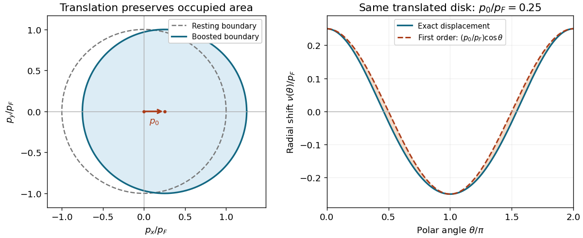
The shifted Fermi circle satisfies $|\mathbf{p}-p_0\hat{\mathbf{x}}|=p_F$. Its radial boundary at polar angle $\theta$ is the positive solution of $p^2-2p{p}_0\cos \theta +p_0^2=p_F^2$. Thus, for $p_0<p_F$,and its leading Taylor expansion isForward-pointing momenta gain occupied states and backward-pointing momenta lose them. With the paper's explicitly reversed Heaviside step function convention, ${\Theta }^{\prime }(x)=-\delta (x)$; consequentlywith a positive leading sign.

For the later quadratic energy calculation it is useful to distinguish the first-order shape from exact particle number conservation. The particle-conserving displacement of a Fermi circle hasThe second-order inward correction cancels the apparent area increase one would obtain by treating $\nu =p_0\cos \theta$ as exact.

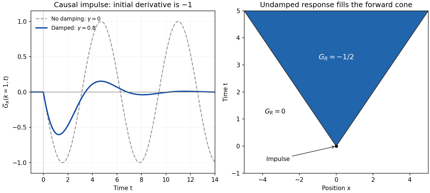
An impulse at $a$ shifts the causal sine response. Substituting the Dirac delta in the convolution from part (i), or using the Laplace transform time-shift rule, giveswhere $H$ is the Heaviside step function. The answer is continuous at $a$, while its first derivative jumps from $0$ to $1$. Consequently its second distributional derivative contains exactly one unit Dirac delta at $a$, giving $f^{\prime \prime }+f=\delta (x-a)$. Since $a>0$, both initial conditions vanish.

By definition, the relaxation modulus is the stress generated by a unit step of strain from an initially relaxed state. Set $ϵ(t)=H(t)$, where $H$ is the Heaviside step function, and write $\sigma (t)=G(t)$. Integrating the linear ordinary differential equation across the step shows that neither $G$ nor $G^{\prime }$ can jump: a jump would produce a Dirac delta function or its derivative, absent from the forcing. Hence $G(0^{+})=G^{\prime }(0^{+})=0$.

For $t>0$, a particular solution is $1$. The characteristic equation factors asso $G=1+A{e}^{-t/5}+B{e}^{-t/3}$. The initial conditions give $A+B=-1$ and $A/5+B/3=0$, whenceThe time and modulus units are those implicit in the printed coefficients. A Laplace transform check gives $\hat{G}(s)=1/[s(5s+1)(3s+1)]$.

The original PDF really does put undifferentiated strain on the right-hand side. The resulting response rises from zero to one, with $G^{\prime }(t)=\frac{1}{2}(e^{-t/5}-e^{-t/3})>0$, rather than exhibiting ordinary stress relaxation. There is a stronger physical problem if this is intended as a passive material law: with the convention $e^{i\omega t}$ the stress-to-strain amplitude ratio isThe loss modulus would give negative cycle-averaged supplied power $⟨\sigma \dot{ϵ}⟩=\omega G^{\prime \prime }|{ϵ}_0{|}^2/2$, contrary to passivity in linear viscoelasticity. The boxed expression is therefore the formal relaxation modulus of the equation as printed, not a claim that this equation describes an ordinary passive viscoelasticity model. No derivative of the input has been silently inserted.

For $0<k^2<4/{\gamma }^2$, defineThe simple poles are ${\omega }_{\pm }=\pm {\Omega }_k-i{a}_k$. In the inverse transform $\tilde{G}(k,t)=\int e^{-i\omega t}\hat{G}d\omega /(2\pi )$, close the contour below for $t>0$. Its clockwise orientation gives $-i$ times the sum of residues. That sum isFor $t<0$, close above; there are no poles. The residue theorem therefore givesHere $\Theta$ is the Heaviside step function. At $k=0$ the continuous retarded limit is $-t\Theta (t)$. At critical damping, ${\Omega }_k\to 0$ likewise replaces $\sin ({\Omega }_{k}t)/{\Omega }_k$ by $t$; beyond the stated oscillatory range an imaginary ${\Omega }_k$ converts it to a hyperbolic sine. These continuations retain decaying temporal exponents.

For each fixed $k$, taking $\gamma \to 0^{+}$ givesFor $t>0$, invert in space and set $s=kt$:The correctly normalized sinc function transform isFor instance, $\sin s/s=\frac{1}{2}{\int }_{-1}^1{e}^{isy}dy$, and Fourier inversion immediately gives the factor $\pi$. The PDF's prefactor $\sqrt{2/\pi }$ is inconsistent with its top hat of unit height; it would give height $\sqrt{2\pi }$. Using the normalized identity yieldsas a distribution. The values assigned precisely at a wave front do not change that distribution. This is the negative of the standard one-dimensional retarded wave Green function, because the PDF's differential operator is $-{\partial }_t^2+{\partial }_x^2$.

The sign and initial data can be checked without any contour calculation. Integrating the spatial-Fourier equation through the impulse givesIn real space these are $G_R(x,0^{+})=0$ and ${\partial }_t{G}_R(x,0^{+})=-\delta (x)$. In particular,for a smooth test function $f$, confirming the negative delta-function initial velocity. Before the impulse the displacement and velocity are zero. The disturbance fills the forward causal cone for the constant-speed wave equation, whose fronts move at unit speed, consistent with $\rho =\kappa =1$. The final question's printed $\rho =k$ is interpreted as $\rho =\kappa$, referring to the elastic constant, not to the Fourier wavevector. No initial conditions were otherwise specified, so the causal choice has been made explicitly.

Put $T=t-t^{\prime }$. momentum eigenstates evolve with energy $p^2/(2m)$, so the retarded momentum kernel is $\theta (T)\delta (p-p^{\prime })e^{-i{p}^{2}T/(2m\hslash )}$. Its Fourier transform reduces toCompleting the square and defining the oscillatory Gaussian integral by a convergent limiting prescription givesFor $T>0$ the square root has quantum phase $e^{-i\pi /4}$. As $T\downarrow 0$, this kernel tends to $\delta (x-x^{\prime })$ in the distributional sense. Differentiating the Heaviside step function consequently supplies the required $i\hslash \delta (T)\delta (x-x^{\prime })$ source; an extra $-i/\hslash$ factor would correspond to a different Green-function convention.

For a time-independent Hamiltonian operator, the time-evolution operator is $U(T)=e^{-iHT/\hslash }$, with $T=t-t^{\prime }$. Insert its resolution of identity in normalized energy eigenstates:Since $⟨x|\alpha ⟩={\phi }_{\alpha }(x)$, the retarded quantum propagator in the question isThe Heaviside step function imposes the chosen retarded convention. If the Hamiltonian operator has a continuous spectrum, the spectral sum includes its continuum integral; it must not be restricted to bound states. The spectral resolution of a quantum propagator also shows that $K$ tends to $\delta (x-x^{\prime })$ as $T\downarrow 0$. With the step factor it obeys $(i\hslash {\partial }_t-H)K=i\hslash \delta (T)\delta (x-x^{\prime })$; the corresponding Green function with a unit delta source is $K/(i\hslash )$.

Occupation and the two-dimensional Fermi energy. For an independent single-particle state, the Fermi-Dirac distribution isThe chemical potential enforces the chosen mean particle number through $N={\sum }_{j}n({\epsilon }_j)$, including spin states in the sum. It is common to all states in particle-exchange equilibrium and must generally change with temperature or field when the total mean number is held fixed. At zero temperature, the distribution becomes a Heaviside step function at the Fermi energy.

Let the sample area be $\mathcal{S}$ and let $g_s$ be its internal spin spin degeneracy. In the continuum limit, filling the disk $k<k_F$ givesThereforeFor spin-half fermions with both spin states available, $g_s=2$ and ${\epsilon }_F=\pi {\hslash }^{2}N/(m\mathcal{S})$; for a spin-polarized gas $g_s=1$. The question does not specify the area or spin degeneracy, so these conventions must be stated rather than extracting an energy from $N$ alone. Although the original text calls $\mathbf{k}$ momentum, the supplied ${\hslash }^2{k}^2/(2m)$ dispersion makes it a wave vector; physical momentum is $\mathbf{p}=\hslash \mathbf{k}$. The result agrees with the constant two-dimensional free-electron density of states. Discrete level spacings in a finite sample would require a specified boundary spectrum.

One level occupied on average. Write $\delta ={\mu }_{B}B$ and $z=e^{\beta (\epsilon -\mu )}>0$. The two mean spin occupations areImposing $N_{+}+N_{-}=1$ gives $2+z(e^{\beta \delta }+e^{-\beta \delta })=1+z(e^{\beta \delta }+e^{-\beta \delta })+z^2$, hence $z^2=1$. Thus, for every positive temperature,The total magnetic moment is $\mathcal{M}=-{\mu }_B(N_{+}-N_{-})$. ConsequentlyThis is the grand-canonical spin susceptibility of a half-filled single level. Empty, singly occupied and doubly occupied orbital states are allowed in the grand canonical ensemble. At zero field, the singly occupied configurations together have probability $1/2$, explaining the factor of two relative to one permanent spin-half moment. If exactly one electron were required at all times, a canonical two-state partition function would instead give $\mathcal{M}={\mu }_B\tanh (\beta {\mu }_{B}B)$ and $\chi ={\mu }_B^2/(k_{B}T)$. That different answer does not implement the stated average-number constraint.

Density-of-states formula for the susceptibility. Here $g$ is the zero-field single-spin density of states. Regard its argument $E$ as the full spin-shifted energy. The shifted functions are $g_{\pm }(E)=g(E\mp {\mu }_{B}B)$, soThe total number is even in $B$; thus $\mu (B)=\mu (0)+O(B^2)$ at fixed total number on a smooth branch. More directly, terms from ${\mu }^{\prime }(0)$ cancel in the spin difference because the two densities coincide at zero field. To first order,It follows thatFor a physical energy band, take $g$ to vanish below its lower edge. Provided the endpoint term vanishes, integration by parts also givesThis form displays the positive response and the narrow thermal window around $\mu$. A sharp band edge is included by the corresponding distributional derivative in the first expression. The susceptibility defined here is the derivative of total magnetic moment with respect to $B$, with units $\mathrm{J}{\mathrm{T}}^{-2}$; it is not automatically a dimensionless SI volume susceptibility. A density-of-states convention per unit volume likewise gives a response per unit volume. These are the field conventions for magnetic susceptibility.

Chemical potential at fixed number. Define the integrated single-spin state countThe probability kernel $K_T$ has unit integral, mean $\mu$, and variance $a(k_{B}T{)}^2$. Using integration by parts,Expand $G$ about $\mu$. The linear term integrates to zero, while $G^{\prime \prime }=g^{\prime }$ givesThis is the number form of the Sommerfeld expansion. Since $N/2=G({\epsilon }_F)$ at zero temperature, set $\mu ={\epsilon }_F+\delta \mu$ with $\delta \mu =O(T^2)$:ThereforeThe coefficient can be obtained directly. With $y=(E-\mu )/(k_{B}T)$,For example, the sum follows by expanding $e^{-y}/(1+e^{-y}{)}^2$ on $y>0$, using the evenness of the kernel and integrating each exponential. Thus $a/2={\pi }^2/6$. A density of states increasing with energy gives a downward quadratic chemical-potential shift. For the constant two-dimensional density of states that shift vanishes to this order; a finite lower band edge still allows exponentially small corrections.

Low-temperature susceptibility at fixed number. Apply the same kernel expansion to $g$ itself:The shift of $\mu$ must be retained in the first term. Writing $g_F=g({\epsilon }_F)$ and similarly for its derivatives,ConsequentlyThis is the fixed-number low-temperature Pauli susceptibility. The $g_F^{\prime \prime }$ contribution is thermal broadening at fixed chemical potential; the $-g_F^{\prime 2}/g_F$ contribution enforces fixed total number. Both are needed. If the density of states were instead defined with both spin directions included, the prefactor $2$ would be absorbed into that definition. Only the spin response has been calculated; no orbital magnetic response is included.

The expansion assumes $g_F>0$, sufficient smoothness near the Fermi energy, and a temperature small compared with the energy scale over which $g$ changes or encounters a band edge. It does not apply unmodified at a singular density of states. For the ideal two-dimensional parabolic band, $g_F^{\prime }=g_F^{\prime \prime }=0$, so the leading Pauli response is temperature independent, consistently with the earlier state count.

Use the Heaviside step function with the value at the jump chosen as follows:For any open set in the target Sorgenfrey line, its preimage is one of $\varnothing$, $\mathbb{R}$, $(-\infty ,0)$, and $[0,\infty )$. All four are open in the source Sorgenfrey line, so $f$ is continuous. In the Euclidean topology, the preimage of $(1/2,3/2)$ is $[0,\infty )$, which is not open. Hence the same function is not continuous as a usual real-to-real map.

A function is piecewise continuous on a finite interval if it is continuous between finitely many breakpoints and has finite one-sided limits at those points and at the endpoints. On $[0,\infty )$, require this on every finite interval. A Heaviside step function is an example; a function with an infinite blow-up at an interior point is not. This condition guarantees local integrability while allowing jumps in an input.

The position-space kernel of the time-evolution operator propagates a wave function by $\psi (x,t)=\int K_U(x,t;x^{\prime },t^{\prime })\psi (x^{\prime },t^{\prime })d{x}^{\prime }$. It tends to $\delta (x-x^{\prime })$ as $t\to t^{\prime }$. A retarded convention multiplies it by the Heaviside step function: $K_R=\Theta (t-t^{\prime })K_U$. This convention obeys $(i\hslash {\partial }_t-H)K_R=i\hslash \delta (t-t^{\prime })\delta (x-x^{\prime })$; dividing by $i\hslash$ gives the Green function with a unit delta source. The time phase for an energy eigenstate is always $e^{-iE(t-t^{\prime })/\hslash }$.

The quasiparticle residue is the coherent pole weight of the single-particle Green's function. Its coherent spectral term $Z\delta (E-{\xi }_p)$ contributes $Z\Theta (-{\xi }_p)$ to the zero-temperature momentum occupation. A smooth remainder leaves a jump $Z$ at the Fermi surface; Landau quasiparticle occupations have a unit step.^[ref]

For the local illustrative distribution in the figure, put $x=(p-p_F)/p_F$ and$\Theta$ is the Heaviside step function. Its one-sided limits are $0.825$ and $0.175$, giving $Z=0.65$. The smooth term is stipulated; this local curve does not specify a normalized distribution over all momenta. In particular, $Z$ is neither the fraction of atoms above the Fermi surface nor $m/m^{\ast }$.

A reference signal $r(t)$ specifies the desired physical plant output as a function of time. A fixed reference signal is often called a setpoint; a changing reference signal describes a trajectory to follow. A reference signal is a goal, whereas the control input $u(t)$ is the command chosen to achieve that goal. ^[ref]

Asking for a temperature of $40{}^{\circ }\mathrm{C}$ does not specify a heater command of $40\%$: dimensional analysis distinguishes the units of these quantities. The reference signal and the measured output must describe the same quantity in the same coordinates before their difference can define a tracking error. An unconverted sensor readout cannot be subtracted directly from a desired temperature.

For example, let $y=T-T_0$ be temperature rise above a fixed ambient baseline $T_0$, and write the desired temperature as $T_d=T_0+r$. A Heaviside step function gives $r(t)=R$ for $t\ge 0$, with $r(t)=0$ before the change: the target rise becomes $R$ at once, although a physical controlled plant generally cannot jump at once. A ramp reference signal $r(t)=vt$ instead asks the temperature rise to increase at a fixed rate $v$. If $R=1{}^{\circ }\mathrm{C}$ and $v=0.2{}^{\circ }\mathrm{C}{\mathrm{s}}^{-1}$, the first reference signal asks for a lasting one-degree rise; the second asks for a one-degree rise at $t=5\mathrm{s}$ and a two-degree rise at $t=10\mathrm{s}$. Here degree Celsius differences are also kelvin differences. A target that grows forever is useful for analytical tests but eventually exceeds a real heater's range.

To make the distinction between a goal and a command concrete, the examples in steady-state tracking error use the first-order low-pass filter as a new controlled plant, rather than the accumulating controlled plant $\dot{x}=u+w$ used in the earlier feedback demonstration:The time constant $\tau$ has units of time, $K$ has units of plant output per control input, and the additive control disturbance $d$ has the units of $y$. This $d$ is an equivalent output offset, not the rate-like $w$ in $\dot{x}=u+w$. A heater interpretation uses $y$ in degree Celsius differences and $u$ in percentage points of heater command, with $K$ in degrees per percentage point; the control input is a command, not a direct measurement of delivered power. With exact measurement, holding $y=R$ requires $u=(R-d)/K$. Thus even a constant reference signal can require a persistent nonzero control input. The numerical model below is deliberately synthetic and has no fitted laboratory parameters.

For $y_{tt}=c^2{y}_{xx}$ on $0<x<L$, initially at rest with zero displacement, apply $y(0,t)=a$ for $t>0$ and keep $y(L,t)=0$. A geometric series in the Laplace transform givesHere $H$ is the Heaviside step function, $L,c>0$, and only finitely many terms contribute at any finite time. The second step in each pair is a sign-reversed reflection from the fixed endpoint. The formula solves the wave equation classically away from the fronts and distributionally across them; the midpoint is a square wave of period $2L/c$.

Signaling adaptation is a decline of a response toward its earlier level while the initiating signal remains present. Specify which response is measured and its baseline: complete signaling adaptation means eventual return to that baseline; partial signaling adaptation leaves a lasting displacement. The continuing signal distinguishes signaling adaptation from simply switching off the stimulus. Signaling adaptation describes behavior, while signaling feedback describes a causal arrangement, so neither implies the other.

By reducing a persistent response to background ligand concentration, signaling adaptation can make a biological cell sensitive to changes rather than only to absolute levels. Resetting the response helps leave room for another change over a useful range of ligand concentrations. This is valuable in chemotaxis: swimming bacteria encounter changing chemical conditions, and their signal transduction influences whether a run continues or a tumble occurs. Signaling adaptation helps separate a change encountered during motion from a lasting background. This usefulness does not imply exact return or equal sensitivity at every possible concentration. ^{[ref] [ref]}

Here is a solvable incoherent feedforward loop toy that exhibits complete signaling adaptation without signaling feedback. The input $s(t)$ jumps from $0$ to $1$ at $t=0$ and remains $1$, a Heaviside step function. Let $x$ be a fast activating branch, $a$ a slower inhibitory branch, and $r=x-a$ a readout. The activities $s,x,a,r$ are dimensionless variables; physical time is in seconds. Choose time constants ${\tau }_x=1$ second and ${\tau }_a=5$ seconds, with initial conditions $x(0)=a(0)=0$:Both branches read $s$ directly. Neither branch depends on $r$, and $a$ does not change $x$: the subtraction only defines the readout. Thus the slow opposing influence is feedforward, with no closed feedback control loop.

For $t\ge 0$, solving the two ordinary differential equations givesWriting $t$ for the numerical time in seconds, these are $x=1-e^{-t}$, $a=1-e^{-t/5}$ and $r=e^{-t/5}-e^{-t}$. Initially $r=0$, then $x$ rises faster than $a$, producing a pulse. At long times $x$ and $a$ both approach $1$, so $r$ returns to $0$ despite sustained $s=1$. For this upward step $e^{-t/5}\ge e^{-t}$, hence $r(t)\ge 0$. The striking feature of this signaling adaptation toy is that both branches remain active while the readout becomes quiet: the continuing background and the response to its arrival are separable.

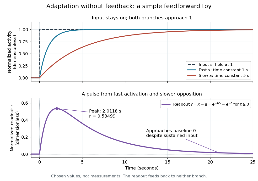
Find the pulse maximum by differentiating the exponential functions. With numerical time in seconds, the derivative isThe stationary condition is $e^{-4t/5}=1/5$, so the natural logarithm givesBefore this time the derivative is positive; afterwards it is negative. Together with $r(0)=0$ and ${\lim }_{t\to \infty }r(t)=0$, this proves that it is the unique pulse maximum. As another numerical check, at $t=10$ seconds $x\simeq 0.999955$, $a\simeq 0.864665$ and $r\simeq 0.135290$: the slow branch is still catching up.

The subtraction $r=x-a$ is a mathematical readout, not a claim that an actual chemical concentration equals this difference for arbitrary inputs. Nonnegativity was established only for the specified upward step; other input histories can give a negative signed readout. Complete signaling adaptation here also relies on equal eventual branch gains: changing the readout to $r=x-0.9a$ leaves $r_{\ast }=0.1$ for $s=1$. This toy illustrates cancellation and different time constants; it does not establish molecular implementation or robustness to arbitrary parameter changes. Ma and colleagues' 2009 study separately analyzed biochemical mathematical models with negative feedback and incoherent feedforward loops, identifying additional conditions for signaling adaptation in those models. ^[ref]

A historical connection to feedback control comes from Yi, Huang, Simon and Doyle's 2000 analysis of a bacterial chemotaxis model. They identified integral action in its regulation of receptor activity: accumulated deviations alter a slower adjustment, which in turn changes the measured activity. At a stationary state, an adjustment that integrates a nonzero error cannot remain constant, explaining how zero error can follow. Their conclusion depended on stated biochemical assumptions and stable behavior; it was not a claim that every biological cell uses that mechanism. A transient pulse alone, as the incoherent feedforward loop toy shows, cannot identify the underlying signaling feedback architecture. ^[ref]

Integrating the smooth positive-time impulse kernel gives the zero-data response to the Heaviside step function. For nonzero $\omega$,At zero frequency and nonzero $k$ the limit is $[1-e^{-kt}(1+kt)]/k^2$; when both parameters vanish it is $t^2/2$. The integral representation avoids ambiguous divisions in these limiting cases.

In coordinates $s=t$, $y=x-t$, the transport derivative $u_t+u_x$ becomes $U_s$. A Heaviside step function moving at that speed becomes stationary, and its twice-integrated profile gives the displayed continuously differentiable solution of $u_t+u_x=u_{xx}+H(x-t)$. Its second spatial derivative has a jump, so the equation holds away from the moving interface and in the distributional sense there.