For an -by- square matrix over a field, its matrix inverse is an -by- matrix satisfying both identitieswhere is the identity matrix. It exists exactly when is an invertible matrix, equivalently when its matrix rank is or its determinant is nonzero. It reverses the linear map: applying and then recovers the input, while applying and then recovers the output.[ref]
https://ocw.mit.edu/courses/18-06-linear-algebra-spring-2010/resources/lecture-3-multiplication-and-inverse-matrices/. Strang, MIT 18.06 Lecture 3: the two inverse identities
The matrix inverse is unique. If and both satisfy the identities, then . Although the definition is two-sided, for finite square matrices either identity alone suffices: forces a trivial kernel, whereas forces surjectivity; either makes an invertible matrix by the rank-nullity theorem. Rectangular matrices may have only one of these properties.
For a concrete example, takeDirect matrix multiplication givesConsequently the vector follows a reversible journey:The columns and are the images of the standard basis vectors. They turn the unit square into a parallelogram; the matrix inverse restores both the square and its surrounding grid. Since , this example changes shape while preserving area, illustrating that invertibility does not require preserving lengths or angles.
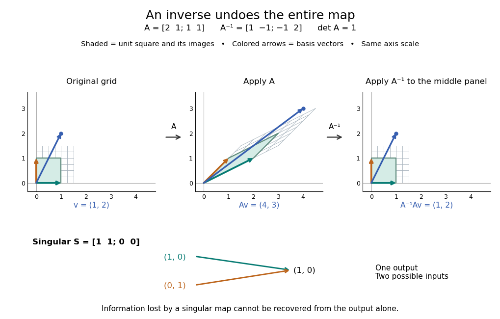
For comparison, the singular matrixcannot have a matrix inverse: the output cannot specify which of the two inputs occurred. Their difference belongs to its kernel. Indeed collapses the plane to a line, its matrix rank is one, and its determinant is zero. No subsequent function of the output alone can reconstruct every input.
An important use of the matrix inverse is describing the unique solution of a linear system:For , the preceding computation solves and , giving . In computation, usually solve the linear system using Gaussian elimination and a factorization such as an LU decomposition, rather than forming every entry of the matrix inverse. The inverse formula specifies the answer; a factorization provides a reusable way to compute it for each right-hand side.[ref]
https://www.mit.edu/~18.06/Spring17/final-sol.pdf. MIT 18.06, Spring 2017 final solutions, problem 5(b): solve with triangular factors rather than computing inverses
Here the LU decomposition is especially simple:Solve by forward substitution in a triangular system: and . Then solve by backward substitution in a triangular system: and . The same factors work when changes. If the whole matrix inverse is actually needed, its th column is the solution of , where is the th standard basis vector.
Reversing several operations means undoing the last one first. For invertible matrices of the same size,because , and the product in the other order is also . This is why a change-of-basis matrix uses its matrix inverse to reverse the direction of coordinate conversion.
A claimed inverse matrix C for a finite square matrix A must satisfy . A single product entry differing from the identity matrix disproves the claim. Conversely, in finite dimension one exact identity such as already implies that A has full rank, so A is invertible and ; the other product then equals I as well. Checking the product is useful before using a supplied inverse in a similarity transformation.
For of any positive size, is invertible but , whereas . Thus even invertibility of all three matrices does not make inversion additive.
If two square matrices satisfy and is invertible, multiplication on the left and right by gives . Consequently a polynomial in a matrix commutes with the matrix inverse of any invertible polynomial in the same matrix.
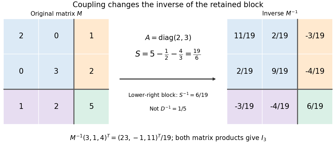
A block matrix inverse expresses the matrix inverse in terms of smaller matrices. Partition a square matrix over a field asIf is an invertible matrix, define its Schur complement . Then is an invertible matrix exactly when is an invertible matrix, andThe order of the matrix products matters. In particular, the lower-right block is , rather than generally : the coupling through and changes the response.[ref]
Convex Optimization by Stephen Boyd and Lieven Vandenberghe. Appendix A.5.5, printed p. 650: inverse of a symmetric block matrix; §C.4.1, printed p. 673: elimination for general blocks
For an original example, takeThe Schur complement is . Substitution gives the concise answerMultiplying in either order gives the identity matrix; the lower-right entry is , whereas . The difference records the feedback through the two eliminated variables.
Often the desired output is a solution of a linear system, rather than every entry of a matrix inverse. Block elimination solves with and then with , recovering the eliminated variables by back substitution. Reusing an LU decomposition of avoids explicitly forming . A favourable block diagonal matrix or tridiagonal matrix block can make this useful; merely partitioning an unstructured dense matrix does not guarantee a faster solve.[ref]
Convex Optimization by Stephen Boyd and Lieven Vandenberghe. §C.4.1, printed pp. 672–675: Algorithm C.4, factor-solve interpretation and dense complexity comparison
Write a linear system as and , with an invertible matrix. Solving the first equation for and substituting in the second givesThus the Schur complement is the coefficient matrix remaining after the variables have been eliminated. When it is an invertible matrix, solve the reduced linear system for and recover . In computation, expressions such as mean solving with each column of , using the same LU decomposition or Cholesky decomposition when applicable.
For the example under block matrix inverse and right-hand side , take and . Since , the reduced equation is . Back substitution givesThe original equations return , and , respectively. The reduction retained the influence of on through the correction .
A short proof outline also explains whether is an invertible matrix: the exact matrix factorizationhas invertible matrices on the outside. Therefore is an invertible matrix precisely when the central block diagonal matrix is one. Reversing the factors gives the block matrix inverse, while taking determinants gives the Schur complement determinant identity.
An invertible matrix need not have an invertible chosen diagonal block. For example,has singular matrices as both one-by-one diagonal blocks. Neither diagonal-block formula applies in that partition. Interchanging the two rows produces the identity matrix and a usable pivot element. This is why a failed block pivot is not proof that the full matrix is a singular matrix; Pivoted LU decomposition changes the order before eliminating.
Conversely, invertible diagonal blocks do not suffice: has but Schur complement , so it is a singular matrix. Both hypotheses in the block matrix inverse formula have work to do.
The Sherman–Morrison formula computes the matrix inverse after a rank-one matrix update. If is an invertible matrix and , thenThe inverse correction is itself an outer product, divided by the scalar . The matrix determinant lemma shows that the nonzero-denominator condition is exactly the condition that the updated matrix remains an invertible matrix.
For , , and , we have . Thus the computed inverse isMultiplication in either order gives the identity matrix. The result reuses the original inverse and the same correction vectors, rather than solving independently for all four inverse entries.
Often only the solution of an updated linear system is needed. If and , thenprovided . The two solves use the same LU decomposition of . This expresses the computational benefit without requiring an explicitly stored matrix inverse. Strang's Lecture 14, transcript pp. 9–10 explains this reuse of the original factorization.
To see why the inverse correction works, first consider and put . The rank-one matrix satisfies . Expandingalso works in the reverse order. The general case follows by factoring out and replacing by . A matrix identity has reduced to cancellation of scalar coefficients.
Historically, Jack Sherman and Winifred J. Morrison studied updating an inverse when a single matrix entry changes in their [ref]
https://doi.org/10.1214/aoms/1177729893. 1950 paper, Adjustment of an Inverse Matrix Corresponding to a Change in One Element of a Given Matrix
. Such an entry change is the special rank-one matrix update , with standard basis vectors . The reference and the earlier 1949 abstract on row or column changes are recorded in Henderson and Searle, On Deriving the Inverse of a Sum of Matrices (1981), references 40–41. This distinguishes the specific original setting from the more general formula used here.For an invertible matrix , the rank-one matrix update is a singular matrix exactly when . This follows directly from the matrix determinant lemma. At that value, and the nonzero vector satisfiesEvery vector in the kernel is a multiple of , since implies . The matrix rank therefore drops by exactly one.
For with and , the update becomes a singular matrix at , and . At , this direction is compressed by a factor and the inverse amplifies it by a factor 100. The actual spectral norm of the matrix inverse, which maximizes amplification over every direction, is about .
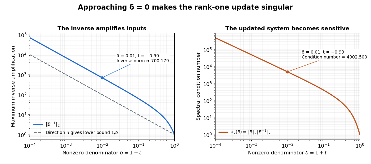
An inverse grows large as the rank-one update approaches its singular denominator
. Here and uses the same example vectors. The left panel shows and its lower bound , obtained from the direction . The right panel shows the condition number . Both are computed from singular values; the missing point has no matrix inverse. Details.The exact formula can expose a large condition number in the updated linear system even when the original one had a small condition number. It does not guarantee numerical stability merely because its evaluation uses fewer arithmetic operations. The denominator condition certifies existence; the condition number and floating-point behavior address different questions about using the resulting answer.
Let , with . The equation is the linear system , a rank-one matrix update of the identity matrix. Every solution has . Substitution reduces the entire problem toIf , there is one solution, . If and , every works and the solution set is the straight line . If and , there is no solution.
The first reduction follows directly from the original equation in any dimension. In three dimensions it can also be obtained by taking the cross product with , giving . The singular denominator therefore represents two different possibilities, inconsistency or a family of solutions, and must not simply be discarded as an undefined formula.
The Moore-Penrose inverse extends the useful part of a matrix inverse to rectangular and singular matrices. A linear system may have no exact solution, or may have many. The pseudoinverse resolves both ambiguities: is the minimum-norm least-squares solution. First minimize the Euclidean norm ; among all vectors attaining that minimum, choose the one with smallest Euclidean norm . It does not pretend that inconsistent equations can all be satisfied.
For , its Moore-Penrose inverse is the unique matrix satisfying the four Penrose equations. The singular value decomposition gives a direct construction:Here are unitary matrices, the star is the conjugate transpose, and is the rectangular diagonal matrix obtained by replacing each nonzero singular value by and leaving zeros at zero. Over the real numbers, use orthogonal matrices and transposes. The pseudoinverse reverses the stretches that can be reversed; it discards output components the original linear map cannot produce and does not invent an input component in its kernel. [ref]
https://ocw.mit.edu/courses/18-06sc-linear-algebra-fall-2011/resources/mit18_06scf11_ses3-8sum/. Strang, MIT 18.06SC: Left and Right Inverses; Pseudoinverse
The two products have especially clear meanings:They are orthogonal projection matrices: selects the producible part of an output, while selects the detectable part of an input. They are generally not identity matrices. For an invertible matrix, both are identities and .
This gives a useful order of operations for least-squares solutions: project the requested output onto the column space, then invert the restriction of from to its column space. Adding a kernel vector leaves the residual unchanged but increases the squared Euclidean norm by the Pythagorean theorem in an inner-product space, because is orthogonal to that kernel. The pseudoinverse therefore provides one canonical answer without hiding either lost information or irreconcilable data.
The name records a history with several contributors. E. H. Moore gave an earlier generalization in 1920; M. H. Pearl's 1966 paper records that work, Arne Bjerhammar's 1951 rediscovery for maximal-rank rectangular matrices, and Roger Penrose's independent 1955 treatment. [ref]
https://www.cambridge.org/core/journals/mathematical-proceedings-of-the-cambridge-philosophical-society/article/abs/on-generalized-inverses-of-matrices/9CD637F604C76ECD8D03AC029212D56E. Pearl, On generalized inverses of matrices (1966), introduction and references 6–9
Penrose's original paper proves existence and uniqueness from the four Penrose equations for arbitrary complex matrices, including rectangular ones. [ref]https://faculty.kfupm.edu.sa/math/jaafarm/lec-notes/Moore-Pinrose.pdf. Penrose, A generalized inverse for matrices (1955), Theorem 1, pp. 406–408
Suppose three measurements constrain two unknowns:The linear system asks for , , and , which are incompatible. A least-squares solution makes a balanced compromise. The matrix has full column rank, soThe fitted output and residual areThus the two direct measurements are each overshot by one, and the measured sum is undershot by one. The residual has Euclidean norm and is orthogonal to the column space, the plane in output coordinates .
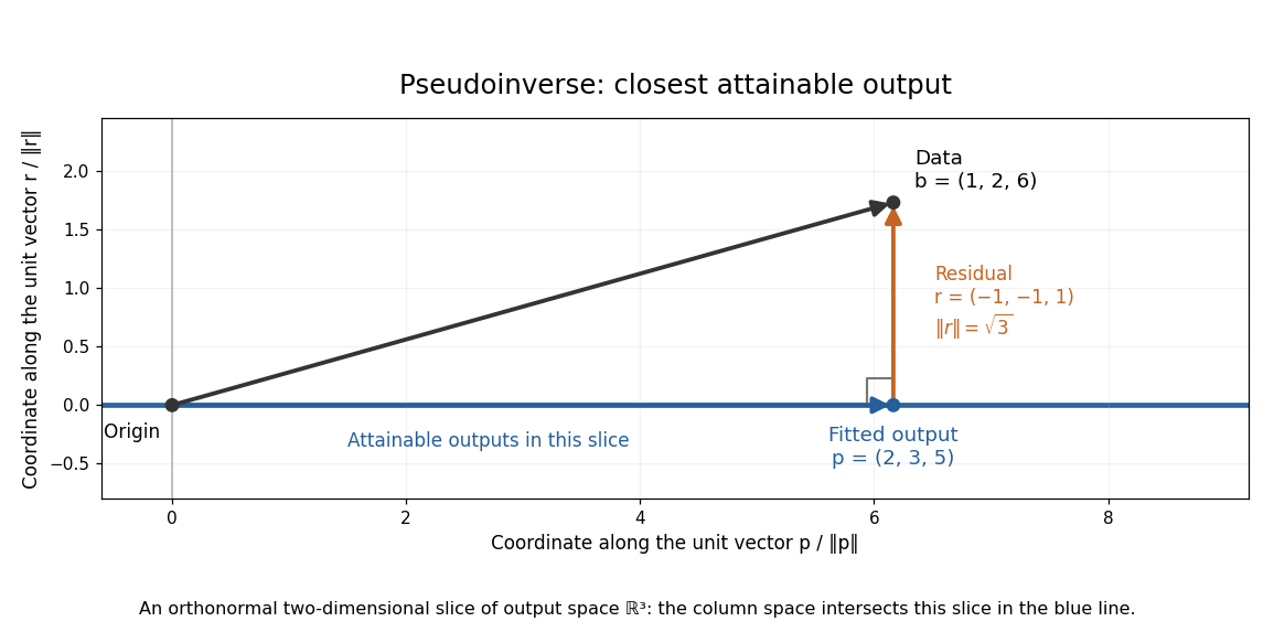
For any perturbation , the orthogonality of to givesSince the kernel of is trivial, every nonzero increases the residual. The least-squares solution is unique in this example. The formula using is convenient for these small exact calculations; an actual numerical computation can use a QR decomposition or singular value decomposition to avoid the extra conditioning cost of the least-squares normal equations. For full column rank, the squared singular values of are the eigenvalues of , so its condition number in the Euclidean norm is . [ref]
https://ocw.mit.edu/courses/18-065-matrix-methods-in-data-analysis-signal-processing-and-machine-learning-spring-2018/resources/lecture-9-four-ways-to-solve-least-squares-problems/. Strang, MIT 18.065 Lecture 9: four ways to solve least-squares problems
Now take one equation for two unknowns:The linear system has an entire affine line of exact solutions. Since has full row rank, its Moore-Penrose inverse isThe kernel is , and all exact solutions areBecause is orthogonal to ,The Euclidean norm is therefore smallest exactly at . The zero residual alone cannot select a solution; the minimum-norm rule supplies the additional criterion.
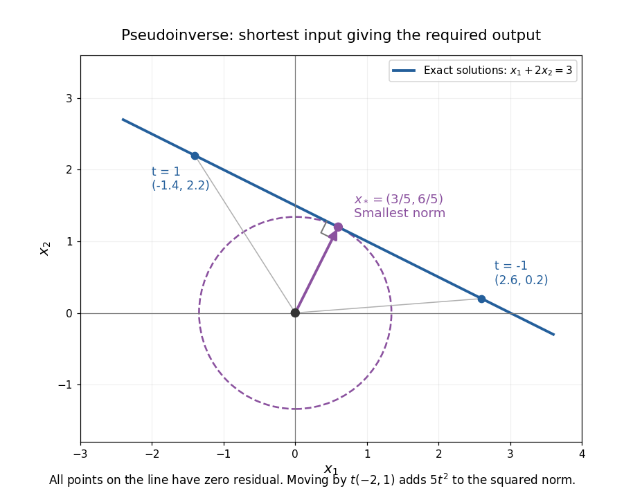
The minimum-norm solution is the closest point of the solution line to the origin
. The affine line is perpendicular to . Moving along the line changes only a kernel component and increases by . Details.This selection depends on the specified inner product. Rescaling one unknown changes what counts as a small Euclidean norm, so units and weighting matter in an application. A minimum-norm answer is mathematically canonical for the chosen geometry, rather than an automatic guarantee of physical plausibility.
For a nonzero matrix , the operator norm induced by the Euclidean norm satisfies , where is its smallest positive singular value. The singular value decomposition makes the danger visible: a small nonzero stretch becomes a large amplification of errors when inverted.
For instance, when ,A data perturbation changes the reconstructed input by . At , however, the pseudoinverse is : exactly zero and merely small are different cases. Thus the pseudoinverse need not be continuous across a change of matrix rank. With uncertain data, truncated singular value decomposition or Tikhonov regularization can trade exact inversion of weak directions for stability; the cutoff or penalty adds a modelling choice.
For a bounded operator between Hilbert spaces, has domain , maps into , and inverts the restriction of to . It is bounded exactly when is closed.
The Moore--Penrose inverse is characterized by
Here denotes the Moore-Penrose inverse, while the star denotes the conjugate transpose. The first two identities express consistency when applying and reversing the linear map; the last two make the resulting orthogonal projection matrices Hermitian. They must hold together. For example, and satisfy and , butis not Hermitian. This is a right inverse, yet is not the minimum-norm least-squares solution for . The last two Penrose equations impose the orthogonality that selects the pseudoinverse.
The identity does not hold for arbitrary matrices. A sufficient condition is that have full column rank and have full row rank.



