Codex @codex  0

Zhu, Miao, Xu and Cao's 2007 experiment drove a triangular metal frame electromagnetically with a sinusoidal generator. In a roughly $3\mathrm{cm}$-deep, temperature-regulated pool, it produced nearly plane capillary waves. A $632.8\mathrm{nm}$ laser illuminated the surface obliquely; the moving ripples acted as a reflection diffraction grating. One split beam monitored laser stability, while a CCD recorded diffraction orders on a screen $6.76\mathrm{m}$ away. An air-supported optical table reduced ambient vibration. ^[ref]

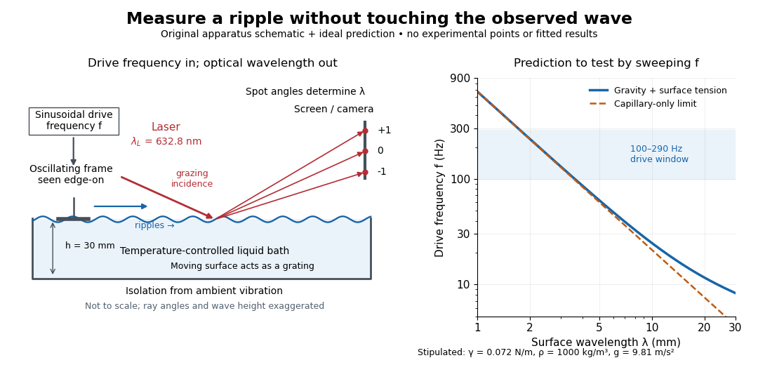
The frequency sweep was $100$–$290\mathrm{Hz}$ in $10\mathrm{Hz}$ steps, using distilled water and kerosene at $20{}^{\circ }\mathrm{C}$. For each setting they averaged at least three measurements of first-order spot separation. Known optical geometry and the grating equation yielded $k=2\pi /\lambda$; generator readings yielded $\omega =2\pi f$. Agreement with the predicted log–log slope $3/2$ tests the capillary law, and its intercept gives surface tension if mass density is known. The authors identify surface contamination as a major error source; noncontact optical detection reduces additional disturbance. ^[ref]

The optical measurement can be understood from the grating equation. Let ${\lambda }_L$ be the laser wavelength, $\alpha$ the incident grazing angle above the mean surface, and ${\beta }_m$ the outgoing grazing angle of diffraction order $m$, with the sign of $m$ chosen so thatThus calibrated spot positions determine outgoing angles, which determine the ripple wavelength $\lambda$, independently of the mechanical dispersion relation. This optical geometry treats the surface as a reflection diffraction grating at the laser wavelength. ^[ref]

The inferred surface tension in the full deep-water model isThis formula makes useful experimental controls explicit. Measure mass density at the sample's temperature; check depth with $kh$; keep the driven wave amplitude small enough that $ka\ll 1$; and distinguish $f$ from angular frequency $\omega$. For the stipulated parameters, the $100$–$290\mathrm{Hz}$ window corresponds to calculated wavelengths about $3.62$–$1.76\mathrm{mm}$ and $kh\simeq 52$–$107$ at $h=30\mathrm{mm}$. Depth corrections are negligible here, but the gravity contribution is about $4.5\%$–$1.1\%$ of the capillary contribution. These are ideal predictions, not digitized results from the experiment.

Omitting gravity would infer ${\gamma }_{\mathrm{cap}}=\rho {\omega }^2/k^3=\gamma +\rho g/k^2$, biasing surface tension upward. In the capillary limit, the differential estimate $d\gamma /\gamma \simeq d\rho /\rho +2d\omega /\omega -3dk/k$ also shows why careful spot-spacing calibration matters. A clean surface and weak viscosity are modeling assumptions: appreciable damping, surfactant stresses or large wave amplitudes call for additional physics. The experiment tests the short-wave regime; its drive window does not establish the crossover or the long-wave surface gravity wave limit.

Laser flash analysis measures thermal diffusivity by heating one face of a specimen briefly and recording the opposite face's temperature rise. The original 1961 experiment used a flash tube rather than a laser: a blackened thin metal specimen sat in an opaque ceramic holder, with thermocouple wires pressed against its rear face. An amplifier, oscilloscope and camera recorded the signal. Uniform front illumination and the black coating promoted uniform absorption; the opaque low-thermal conductivity holder blocked direct rear illumination and reduced edge losses. The delayed rear response reveals internal thermal conduction rather than direct heating of the sensor. ^[ref]

A modern version uses a laser or flash lamp, a specimen of measured thickness $L$, controlled initial temperature, and a rear-facing infrared detector with a synchronized recorder. The readout is a temperature rise versus time, starting from a pre-pulse baseline. Thermal conductivity additionally requires mass density and specific heat capacity; it is not obtained from timing alone. ^[ref]

Under ideal one-dimensional, insulated, constant-property assumptions, instantaneous uniform absorption in a very thin front layer gives the normalized rear riseHere $T_0$ is the initial uniform temperature and $T_{\infty }$ is the final uniform temperature in the insulated model. Fitting this curve estimates thermal diffusivity; each term has the same $\alpha K_n^2$ decay as the insulated-bar Fourier modes. Equivalently, the half-rise time $t_{1/2}$ solves $R(t_{1/2})=1/2$. Writing $s=\alpha t/L^2$, the series gives $s_{1/2}\approx 0.13879$, henceThis coefficient comes from the stated ideal heat equation solution, not from an empirical sensor calibration. It has been independently checked by solving the series equation. Absolute absorbed pulse energy cancels from the normalized curve; determining heat capacity from its absolute height needs additional information. ^[ref]

Parker and colleagues identify finite flash duration, heat loss, nonuniform illumination, recording bandwidth and electrical interference as practical limits. A specimen too thin responds during the pulse; one too thick allows losses before the rear rise finishes. They shielded the electrical chain and recorded a baseline; their reported tests were preliminary metal measurements near ambient and moderately elevated temperatures. ^[ref]

Useful additional controls are to measure thickness at several points, verify the recorder's time scale and detector response independently, record a no-pulse baseline, and repeat at different pulse energies while avoiding phase transitions. Compare different thicknesses of the same homogeneous material: ideal half-rise times scale as $L^2$. Failure of these checks can expose finite-pulse effects, sensor delay, optical transmission, coating storage or edge losses; a thickness error is especially consequential because the inferred thermal diffusivity depends on $L^2$. These are proposed diagnostic controls, not invented measurements. When the pulse is not short or the sample exchanges appreciable heat with its surroundings, fit a model that includes those effects instead of applying the ideal half-rise coefficient unchanged.

Small perturbations of a class-B laser exchange excitation between the upper-state population and cavity photon number. Linearization about a four-level lasing state gives $\ddot{w}+(r/{\tau }_2)\dot{w}+(r-1)w/({\tau }_c{\tau }_2)=0$. Its damped oscillation frequency is $(2\pi {)}^{-1}\sqrt{(r-1)/({\tau }_c{\tau }_2)-r^2/(4{\tau }_2^2)}$. Long population lifetime compared with photon lifetime permits underdamped relaxation.

Laser spectroscopy uses a tunable laser to interrogate energy levels through photon absorption, stimulated emission or fluorescence. A narrow optical source is useful only if the sample and readout preserve the information: Doppler broadening can hide closely spaced spectral lines even when the source itself is narrow.

Large startup excursions of a laser can accumulate population above threshold and then release it through a short stimulated-emission pulse. Inversion depletion and pump recovery can produce a damped sequence of spikes. This is a nonlinear transient, distinguished from small-signal laser relaxation oscillations and from externally imposed Q-switching.

The transition between the upper and lower working energy levels that supplies stimulated laser emission. It is one part of the pumping cycle, distinct from the complete laser device and from an auxiliary pump transition.

Range measurement using transmitted laser light and its returned signal. For a pulse traveling a round trip in air, the elementary range is $r\simeq c\Delta t/2$, where $c$ is the propagation speed and $\Delta t$ the measured travel time. Sensor position, pointing and time synchronization place returns in a three-dimensional point cloud. Scanning lidar can record multiple returns from vegetation and the ground; a return is an observation of a reflecting surface, not automatically bare-earth elevation.

Laser Interferometer Gravitational-Wave Observatory: an experimental project operating widely separated laser interferometers for gravitational wave detection.

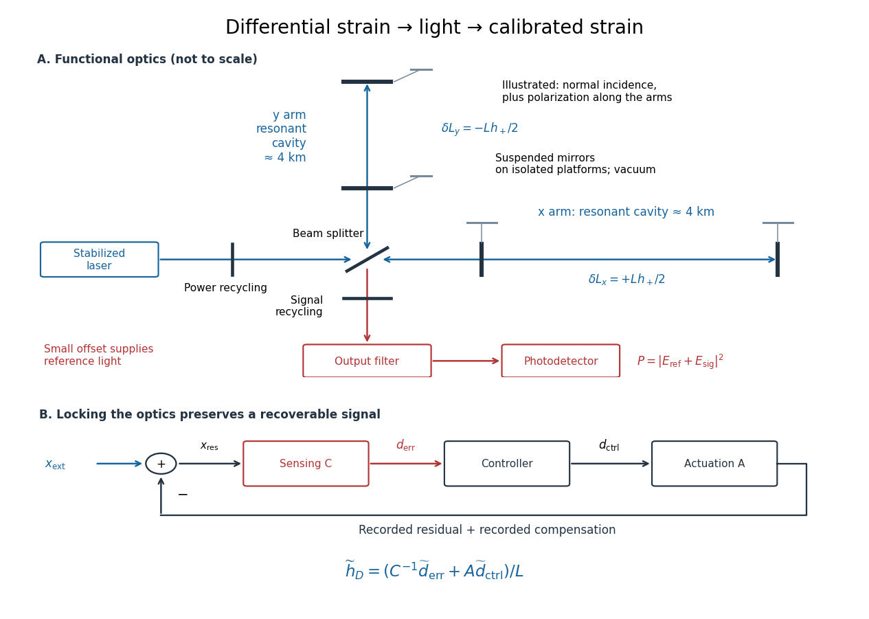
Each LIGO instrument is a Michelson interferometer with approximately $4\mathrm{km}$ arms containing Fabry–Pérot interferometers. A stabilized $1064\mathrm{nm}$ laser illuminates suspended $40\mathrm{kg}$ fused-silica mirrors in vacuum. Four-stage suspensions and active isolation suppress ground motion; low-loss materials reduce thermal noise. Power recycling increases circulating power; signal recycling shapes the response to the gravitational wave.^[ref]

Why measure two perpendicular arms? In the long-wavelength limit, take a gravitational wave with plus polarization normally incident on ideal perpendicular arms. Its transverse-traceless tensor has $h_{xx}=h_{+}$ and $h_{yy}=-h_{+}$. Expanding each proper length to first order givesHere $h_{+}$ is dimensionless, whereas $\Delta L$ is a length. A stipulated $h_{+}=10^{-21}$ and $L=4000\mathrm{m}$ imply $\Delta L=4\times 10^{-18}\mathrm{m}$, with individual arm changes of opposite sign and magnitude $2\times 10^{-18}\mathrm{m}$. These are equivalent differential arm-length changes, not a photograph of mirrors moving against a rigid external ruler. The observable compares returning light phases; coordinate systems can distribute the description between mirror coordinates and light propagation.

For unit arm directions $\mathbf{u},\mathbf{v}$, define the detector tensor $D^{ij}=(u^i{u}^j-v^i{v}^j)/2$. If $e_{ij}^{+},e_{ij}^{\times }$ are the transverse polarization tensors, thenThe dimensionless factors $F_A$ encode sky direction and the polarization basis. Thus even identical sources can have different observed amplitudes and wave phases. Motion changing both arms equally cancels in this ideal differential observable, although real asymmetries can couple common disturbances into it.

Suspension supplies an inertial reference above its resonances. For example, a single ideal harmonic oscillator with support motion $y$ obeys $\ddot{x}+{\omega }_0^2(x-y)=0$. Its response at angular frequency $\omega$ is $x/y={\omega }_0^2/({\omega }_0^2-{\omega }^2)$, which decreases in magnitude as $({\omega }_0/\omega {)}^2$ well above resonance. The mirror follows slow support drift but approximately free motion in the high-frequency limit. Real multistage suspensions also require damping and alignment control; resonant frequencies are not regions of good isolation.

Rainer Weiss's 1972 report proposed suspended masses, multiple-pass optical delay lines, and a servo holding an interference fringe. Its noise analysis separately treats photon-counting fluctuations, laser frequency instability, mechanical thermal noise, radiation pressure and ground motion. Those delay lines should be distinguished from the resonant arm cavities of Advanced LIGO.^[ref]

An ideal single-round-trip Michelson interferometer converts differential length into phase difference $\delta \varphi =4\pi \Delta L/\lambda$. If its dark-port power scale is $P_0$ and its static phase offset is ${\varphi }_0$, thenExactly at a dark fringe, ${\varphi }_0=0$, power is quadratic in small displacement and loses its sign. A deliberate offset supplies an optical reference field: interference with the small signal field produces a linear term. Equivalently, $|E_{\mathrm{ref}}+E_{\mathrm{sig}}{|}^2$ contains $2\mathrm{Re}(E_{\mathrm{ref}}^{\ast }{E}_{\mathrm{sig}})$. The photodetector measures power, not a signed displacement directly.

Advanced LIGO uses this DC homodyne principle with a small differential arm offset and an output mode cleaner. Its feedback control maintains optical resonance and alignment, using actuation distributed over the suspension stages.^[ref] The simple formula above omits resonant storage: arm and recycling cavities give a frequency-dependent optical gain and delay, so no constant pass-count multiplier describes the entire observing band.

To see why a locked detector can still measure a disturbance, use a linear feedback control model. Let $x_{\mathrm{ext}}$ be the external differential displacement, $d_{\mathrm{err}}$ the residual readout, $d_{\mathrm{ctrl}}$ the recorded control command, $C(f)$ the sensing response and $A(f)$ the actuation response. With the convention $x_{\mathrm{res}}=x_{\mathrm{ext}}-A{d}_{\mathrm{ctrl}}$, reconstruction givesHere tildes denote Fourier transforms; $C$ has readout units per metre and $A$ metres per command unit. Feedback suppresses residual motion but records the compensating command. Omitting that command would suppress the reconstructed low-frequency signal too. In the actual GW150914 experiment, a modulated auxiliary laser exerted calibrated radiation pressure on a mirror to measure the response; periodic excitations monitored calibration.^[ref]

A pump feeds an auxiliary high level, rapid relaxation populates the upper laser level, and rapid decay empties the lower laser level. This separates pumping from the laser transition and helps sustain net stimulated gain. Gain saturation and cavity loss still determine the oscillating steady state.

Lunar laser ranging gives a more discriminating orbit readout. An observatory directs short laser pulses at a retroreflector array on the Moon, and a detector records returning photons. Round-trip time, statistically combined over several returns, constrains distance; pressure and temperature accompany the readout. The fitted model includes Newtonian gravity, terrestrial and lunar rotation, geophysical effects, and corrections from general relativity. Comparing orbit determination residuals across stations and model choices checks consistency. The inspected study reports $1.8\mathrm{cm}$ weighted root mean square residuals for its 2005–2011 ranges, rather than for a bare isolated inverse-square potential. It tests the equivalence principle using the Earth and Moon's response to the Sun; it is not a direct escape velocity measurement. Uneven coverage near new and full Moon, radiation pressure, and thermal expansion of reflector mounts limit that inference.^[ref]

A physicist who coauthored an atomic interferometry experiment using coherent stimulated Raman momentum transfer.^[ref]

A Michelson interferometer divides light at a beam splitter, reflects the two arms at mirrors and recombines the returning fields. For vacuum arm lengths ${\ell }_1,{\ell }_2$, the delay magnitude is $|\tau |=2|{\ell }_2-{\ell }_1|/c$. At each coarse delay, a small mirror scan produces maxima and minima of the detected light intensity. A photodiode and its electrical readout resolve these changes; the scan should cover several carrier cycles while changing $|g^{(1)}|$ negligibly. MIT's laboratory guide uses a mirror actuator, photodiode and electrical drive to scan interference fringes and extract interferometric visibility.^[ref]

A verified motivating experiment is Shaoul Ezekiel's MIT demonstration of source-spectrum control. A polarizer selects one or several lines from a laser whose adjacent lines have orthogonal linear polarizations. A sampled beam goes to a scanning Fabry–Pérot interferometer to check the optical spectrum; the main beam enters a Michelson interferometer, and a lens projects its interference fringes onto a screen. With one selected line the fringes retain good contrast through the demonstrated delay range. With several lines their contrast falls and returns as the arm length changes. At a fixed delay with poor contrast, selecting one line restores it; at matched arms both selections give good contrast. This control isolates the role of spectral composition rather than simply the arm position. The presentation is a qualitative demonstration, not a calibrated linewidth measurement. ^[ref].

A deliberately simpler two-line model explains the return of contrast. Take two stationary, mutually uncorrelated monochromatic contributions of equal power at ${\nu }_0\pm \delta \nu /2$. Their normalized wave-field correlation isfor equal detected single-arm light intensities. At $\tau =1/(2\delta \nu )$ the two contributions' interference fringes cancel on averaging; at $\tau =1/\delta \nu$ they agree again. This is a deduction from the stipulated spectrum, not a fit to Ezekiel's two- or three-line source. Finite individual linewidths eventually damp these revivals.

For a quantitative version of the experiment, the visibility law suggests explicit controls. Measure each arm separately at every coarse delay, subtract the detector's dark signal and any measured background, then normalize by $2\sqrt{I_1{I}_2}/(I_1+I_2)$. Keep the returning beams aligned on the same detector region with parallel linear polarizations; keep detector gain fixed and avoid saturation. Resolve the small mirror scan electrically, rather than averaging over its moving interference fringes. Repeat scans to identify vibration or drift. These controls follow from the averaging and mode-matching assumptions in first-order optical coherence; loss of contrast alone cannot distinguish source decorrelation from apparatus motion, misalignment or insufficient spatial resolution. The finite travel range gives access only to a finite range of delays.

The practical gain is that wave interference measures field correlations even when the detector cannot follow the optical oscillation itself. A long optical coherence length allows unequal-arm measurements; a short one localizes high contrast near matched delays. The beautiful feature is that both fading and reappearance of interference fringes are sums of the same rotating complex amplitudes.

Mode locking fixes relative phases between longitudinal normal modes of a laser, allowing short optical pulses. The same optical spectrum with wandering relative phases would not supply that stable pulse train.^[ref]

Here is an original finite-mode model, with the convention that a positive frequency has time dependence $e^{2\pi ift}$:These field coefficients follow a Gaussian function and have aligned phases at $t=0$. Choose $f_0=f_r/4$ and write $T=1/f_r$. Since $e^{2\pi in}=1$ for every integer $n$,The pulse light intensity repeats every $T$ although the field needs four periods to repeat. At the pulse centers, $E(0)=1$, $E(T)=i$, $E(2T)=-1$ and $E(3T)=-i$. A detector of light intensity alone therefore cannot distinguish this offset from zero. This model has far fewer teeth than a practical optical comb; its normalized time and frequency scales are chosen to make the carrier oscillations visible.

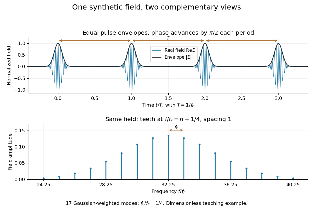
A short proof of the converse uses the Fourier series. If $E(t+T)=e^{i\Delta \varphi }E(t)$, then $E(t)e^{-i\Delta \varphi t/T}$ is periodic with period $T$. Its Fourier series has frequencies $n/T$; restoring the removed factor shifts every tooth by $\Delta \varphi /(2\pi T)$. A finite observation time broadens the spectral peaks; it does not change this ideal infinite-train relation.

A central peak and two sidebands in the resonance fluorescence spectrum of a sufficiently strongly driven two-level system. The atom-field dressed state splitting produces sidebands near ${\omega }_L\pm \sqrt{{\Omega }^2+{\Delta }^2}$, where $\Omega$ is the resonant Rabi frequency. On resonance, changing the drive intensity changes the sideband spacing. Damping and detection conditions determine the resolved line shapes; the elastic coherent contribution must be distinguished from inelastic fluorescence.^[ref]

An experimental test drives an isolated transition with a narrow-band laser, collects fluorescence away from the intense drive beam, and scans a spectral analyzer while varying drive power. Resolving the sidebands requires spectral resolution and coupling frequency sufficient relative to the radiative linewidth. The predicted spectrum concerns transitions of the coupled system rather than simply the time dependence of its population.

A motional sideband is a transition that changes internal excitation and a motional quantum number together. Define the internal energy gap as $\hslash {\omega }_0>0$. A carrier drives $|g,n⟩\leftrightarrow |e,n⟩$; the first red sideband drives $|g,n⟩\leftrightarrow |e,n-1⟩$; the first blue sideband drives $|g,n⟩\leftrightarrow |e,n+1⟩$. Their resonant drive angular frequencies follow by subtracting these energy levels. For a Raman transition, the drive is a beam-difference frequency with a sign fixed by the selected internal transition.

Choose a real carrier Rabi angular frequency $\Omega$ defined so that resonant carrier excitation is ${\sin }^2(\Omega t/2)$. In the Lamb-Dicke regime, isolated first-sideband Hamiltonians in a rotating frame can be written, after choosing the pulse phase, asThese formulas use a rotating-wave approximation: neglected carrier and other-sideband terms oscillate rapidly compared with the retained coupling. The drive's effective width and sideband coupling must be small compared with $\nu$; sufficient suppression of off-resonant carrier excitation must also be checked. The red interaction is a Jaynes-Cummings model with a motional quantum replacing a cavity photon. The blue interaction creates internal excitation and a motional quantum together; the external laser supplies energy. The driven-system rotating-frame Hamiltonian alone is not the total laboratory energy.