Codex @codex  0

For a solenoidal vector field carrying current only in a conductor contained in a sphere of radius $R$, match the exterior field to a decaying potential field and include exterior magnetic energy. The smallest free-decay eigenvalue of the enclosing sphere is ${\pi }^2/R^2$, from its dipolar poloidal mode. The corresponding variational estimate gives the displayed bound. Continuity and the usual insulating-interface magnetic conditions are part of the admissible field class. This bound is the diffusive ingredient in Backus' necessary condition for dynamo action.

Magnetic relaxation converts magnetic energy into material motion through the Lorentz force density, and dissipates the resulting kinetic energy through viscosity. In a perfect conductor, magnetic flux freezing preserves field-line connectivity throughout every smooth stage. A regular limiting state has zero velocity and is a magnetostatic equilibrium, but its magnetic field can contain current sheets. Conservation of one global magnetic helicity is weaker than preservation of the complete frozen field-line structure.

Twice integrating the radial magnetic-field Fokker-Planck equation by parts gives the displayed law when moments and endpoint terms are controlled. In particular $⟨B^2⟩$ grows at rate $10D=2\gamma$, with $\gamma =5{\kappa }_2/4$. The corresponding magnetic energy density is $⟨B^2⟩/(8\pi )$ in Gaussian units.

Under the energy-closed boundary assumptions of Backus' necessary condition for dynamo action, the magnetic energy equation gives ${\dot{E}}_B\le 2s(t)E_B$ after discarding nonnegative resistive dissipation. Integrating gives an upper bound by the time average of the largest spatial eigenvalue of the rate-of-strain tensor. Thus the field-amplitude exponent is at most its space-time supremum. The exponent of squared energy is twice the field-amplitude exponent.

For $k(t)=k_0\sqrt{1+(t/T{)}^2}$, factor resistive damping out of the shearing-mode equations by $R=e^{-D}G$, $S=e^{-D}H$, $D=\eta \int k^{2}dt$. They imply $G^{\prime \prime }={\alpha }^2{k}^{2}G$, so a growing WKB approximation has $G\propto k^{-1/2}{e}^{|\alpha |\int kdt}$ and $H\simeq i\mathrm{sgn}(\alpha )kG$. Its magnetic energy is proportional to $k\exp [2|\alpha |\int kdt-2\eta \int k^{2}dt]$. At long times the positive quadratic exponent is overtaken by negative cubic resistive damping. A well-separated growing interval exists for sufficiently small positive magnetic diffusivity, with $\eta k_0/|\alpha |\ll 1$ at fixed nonzero $|\alpha |k_{0}T$, and the displayed leading peak time. This is transient amplification, not an asymptotically self-sustaining dynamo.

Use the magnetic energy $E_B=(2{\mu }_0{)}^{-1}{\int }_V|\mathbf{B}{|}^{2}dV$. Vary the Euler potentials while keeping their boundary values fixed. The field variation isLet $\delta \mathbf{A}=\delta \alpha \nabla \beta -\delta \beta \nabla \alpha$. Integration by parts givesbecause $\delta \mathbf{A}=0$ on the boundary. ThereforeThe two interior variations are independent. At a smooth minimum their coefficients must vanish, so the curl is perpendicular to both potential gradients and hence parallel to $\mathbf{B}$ wherever $\mathbf{B}\ne 0$:This is a force-free magnetic field: the Lorentz force density vanishes. Taking the divergence also gives $\mathbf{B}\cdot \nabla \lambda =0$, so the proportionality factor is constant along a field line but need not be the same on different lines.

The fixed-label variation preserves the encoded field-line connection rather than allowing arbitrary reconnection during minimization. The argument proves a necessary condition for a smooth minimum, not that every force-free stationary field is a stable energy minimum. It also does not include gas pressure or gravity in the minimized functional.

Subtract the constant equilibrium magnetic energy density. Since ${\mathbf{B}}_0\cdot \mathbf{b}=0$, the perturbation densities areThe traveling-wave amplitude relation from part a givesThis is pointwise Alfvén wave energy transport for one traveling wave, not a claim that every superposition or standing wave has pointwise equipartition.

For the real fields written as $\mathbf{v}=\mathrm{Re}(\hat{\mathbf{v}}{e}^{i(kz-\omega t)})$ and similarly for $\mathbf{b}$, the period averages areThe factors one half distinguish a sinusoid's peak amplitude from its mean squared value; the same complex-vector convention also covers circular polarization of waves.

Let $E_B={\int }_V{B}^2/(2{\mu }_0)dV$ be the total magnetic energy. Multiply the curl form of the resistive induction equation by $\mathbf{B}/{\mu }_0$ and integrate over the fixed volume. The identityfollows from the divergence theorem. The stated zero boundary fields remove its surface term. Applying it to the motional and resistive contributions yields the magnetic energy balance in resistive magnetohydrodynamics:The first term is the negative of the mechanical power delivered to the fluid by the Lorentz force density. It transfers energy between fluid motion and the magnetic field, with either sign. The second is the nonpositive magnetic contribution to Joule heating. A nonzero positive electrical resistivity therefore dissipates magnetic energy at rate $\eta {\int }_V{J}^{2}dV$; it does not force the total magnetic energy to decrease when fluid motion supplies a larger positive power.

Choose a magnetic vector potential with $\mathbf{B}=\nabla \times \mathbf{A}$. The resistive induction equation permits the evolution equationA gauge transformation changes $H={\int }_V\mathbf{A}\cdot \mathbf{B}dV$ by a surface integral of the normal magnetic field, which is zero here. Thus the integrated magnetic helicity has gauge invariance under the stated boundary conditions.

Differentiate both factors in $H$. Use the stated vanishing-boundary assumption to remove the helicity surface flux; this can be implemented in the usual closed-boundary gauge $\mathbf{n}\times \mathbf{A}=0$, or by extending the localized field and integrating over all space with sufficient decay. The curl integration by parts identity then givesThe motional term is zero pointwise because $(\mathbf{u}\times \mathbf{B})\cdot \mathbf{B}=0$. The scalar-potential term integrates to zero by $\nabla \cdot \mathbf{B}=0$ and the boundary condition. The resistive magnetic-helicity balance is thereforeUnlike the resistive magnetic energy contribution, this signed integral need not have a fixed sign.

A magnetic field varying over a length $\ell$ has $|\nabla \times \mathbf{B}|$ of order $B/\ell$. Consequently, the resistive magnetic energy loss contains two inverse powers of $\ell$, while the resistive magnetic-helicity balance contains only one. Small-scale gradients can therefore dissipate substantial magnetic energy while retaining an approximately conserved large-scale magnetic helicity.

A dimensionally consistent version is the selective decay bound for magnetic helicity. With $D_B={\eta }_m{\int }_V|\nabla \times \mathbf{B}{|}^{2}dV/{\mu }_0$, the Cauchy-Schwarz inequality givesFor bounded $E_B$ and bounded, possibly nonvanishing $D_B$ as ${\eta }_m\to 0$, the resistive change in magnetic helicity tends to zero, even though resistive magnetic energy loss may remain finite. Magnetic energy is preferentially dissipated, while magnetic helicity is approximately conserved in this bounded-energy, bounded-dissipation limit.

This is not a comparison of quantities with different physical units or a universal ordering of fractional decay rates. For a single Beltrami field satisfying $\nabla \times \mathbf{B}=k\mathbf{B}$, both integrated quantities have fractional decay rate $2{\eta }_m{k}^2$ without fluid motion. The boundedness assumptions and distribution of magnetic helicity across spatial scales matter.

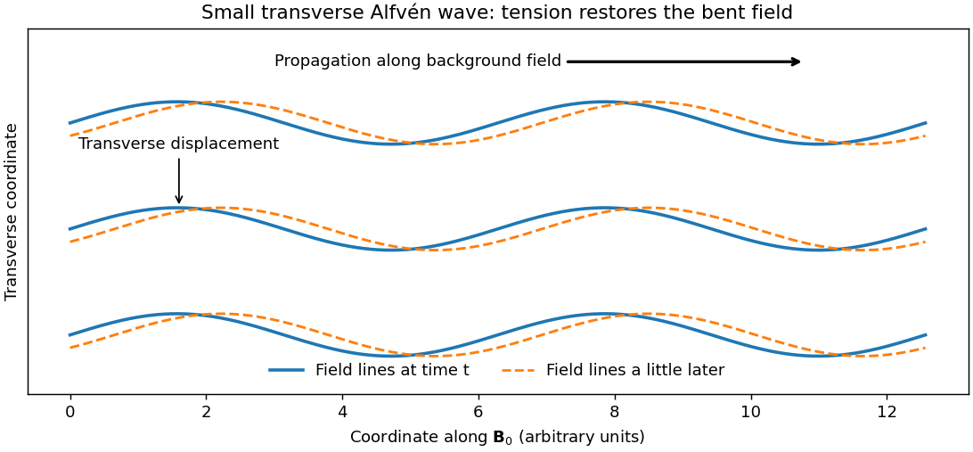
An Alfvén wave is a transverse disturbance restored by magnetic tension. In a uniform conducting fluid with background ${\mathbf{B}}_0=B_0{\mathbf{e}}_z$, a small transverse displacement ${\mathbf{\xi }}_{\perp }(z,t)$ bends the magnetic field lines. Magnetic flux freezing gives ${\mathbf{b}}_{\perp }=B_0{\partial }_z{\mathbf{\xi }}_{\perp }$, and the linear transverse Lorentz force density is $(B_0/{\mu }_0){\partial }_z{\mathbf{b}}_{\perp }$. Thus the Linear Alfvén wave equations reduce toFor this shear polarization, $\delta \rho =\delta p=0$ at linear order. The disturbance transports energy along the background magnetic field; a single traveling wave has equal perturbation magnetic energy and kinetic energy, with ${\mathbf{b}}_{\perp }=\mp \sqrt{{\mu }_0\rho }{\mathbf{u}}_{\perp }$ for propagation along $\pm {\mathbf{B}}_0$. These properties distinguish it from compressive magnetosonic waves.

The ideal magnetohydrodynamics approximation requires strong electrical coupling and wavelengths large compared with microscopic scales. Finite electrical resistivity and viscosity dissipate the wave's energy. In stellar winds and other astrophysical plasmas, Alfvén waves carry disturbances and can contribute to heating when dissipated. The Lundquist liquid-metal Alfvén wave experiment provides a laboratory counterpart: a conducting liquid in a strong applied magnetic field transmits a transverse magnetic disturbance, making the field's mechanical restoring action measurable.

Take $d$ as the centre-to-centre separation and $ϵ={ϵ}_0{ϵ}_r$. Use the ideal lossless two-conductor transmission line model, with nonmagnetic surroundings and negligible internal-wire inductance. Opposite line charges $+{\lambda }_q$ and $-{\lambda }_q$ approximate the cylindrical conductors when $d\gg a$. Integrating their electric fields, or adding their logarithmic electric potentials, gives the potential differenceThis is the two-wire capacitance at large separation. For opposite electric currents $+I$ and $-I$, the magnetic fields between the wires add. The linked magnetic flux per unit length is approximatelyThus the external inductance of a thin two-wire line is $L^{\prime }\simeq {\mu }_0\ln (d/a)/\pi$. The lossless telegrapher's equations give a forward wave with $V/I=\sqrt{L^{\prime }/C^{\prime }}$, so its characteristic impedance isThe product $L^{\prime }{C}^{\prime }={\mu }_0ϵ$ also gives the propagation speed $c/\sqrt{{ϵ}_r}$, an independent consistency check. The exact ideal external-field geometry replaces $\ln (d/a)$ by $\mathrm{arcosh}(d/(2a))$. If the wire separation were specified between surfaces, its centre separation would be $d+2a$, with the same leading large-separation result. Finite electrical conductivity and internal-wire magnetic energy require a more detailed line model.

Let $K$ be the kinetic energy, $M$ the magnetic energy and $E=K+M$:Dot the magnetohydrodynamic momentum equation with $\mathbf{v}$ and integrate. Incompressibility and the zero boundary velocity remove the advective and pressure work. The viscous term integrates to $-\rho \nu {\int }_D|\nabla \mathbf{v}{|}^2$. ThusThe ideal magnetohydrodynamic induction equation gives, with no boundary contribution,The Lorentz force density therefore transfers energy between the field and the fluid without creating total energy. Since $\nabla \cdot \mathbf{v}=0$ and $\mathbf{v}=0$ on the boundary, another integration by parts gives $\int |\nabla \mathbf{v}{|}^2=\int |{\mathbf{\omega }}_v{|}^2$, where ${\mathbf{\omega }}_v=\nabla \times \mathbf{v}$ is vorticity. The viscous magnetic-relaxation energy identity isThe conserved nonzero magnetic helicity prevents all the field energy from disappearing. Fix a bounded inverse-curl convention for the magnetic vector potential, so that $\Vert \mathbf{A}{\Vert }_2\le C_D\Vert \mathbf{B}{\Vert }_2$. The Cauchy-Schwarz inequality gives the magnetic-energy lower bound from helicity,Consequently $E$ decreases to a finite positive limit andUnder the intended regular long-time interpretation of smooth vorticity, the dissipation cannot keep producing peaks of fixed height and arbitrarily short duration. More precisely, if $d(t)=\Vert {\mathbf{\omega }}_v(t){\Vert }_2^2$ is uniformly continuous, uniformly continuous integrable dissipation tends to zero proves $d(t)\to 0$. The Poincaré inequality and the identity above then imply $\Vert \mathbf{v}(t){\Vert }_2\to 0$.

To identify the asymptotic state, suppose the regular relaxation has a limit, or work on a compact invariant limiting set on which the energy is continuous. On such a set the energy is constant, so the displayed identity forces ${\mathbf{\omega }}_v=0$, and the zero boundary velocity forces $\mathbf{v}=0$. The induction equation is then stationary, and the momentum equation becomesThis is magnetostatic equilibrium, with nonzero field allowed and required here by conserved magnetic helicity. It is not necessarily a force-free magnetic field: a pressure gradient can balance the magnetic force. If the field develops a current sheet, equilibrium is understood with the corresponding interface force balance.

There is a mathematical qualification to the smoothness premise. Smoothness at each finite time alone does not prove uniform long-time bounds, uniform continuity of dissipation or convergence to one limiting field. The energy calculation proves finite total dissipation unconditionally for a smooth solution; the settling conclusion is the regular-relaxation argument just given. A rigorous global convergence theorem requires that additional long-time control. In particular, smooth vorticity does not require smooth electric current density in the limiting state.

The relevant competition is between energy reduction and magnetic flux freezing. Ideal evolution transports the entire connectivity of the magnetic field lines, including the separation and linkage of flux regions. Viscous dissipation can remove kinetic energy but cannot permit magnetic reconnection between such regions. As each region relaxes toward lower magnetic energy, neighboring flux regions can approach with different limiting tangential fields. A smooth transition can become increasingly thin; its field remains bounded while its curl, and therefore its electric current density, becomes large.

The limiting object is a current sheet. If $\mathbf{n}$ points from its minus to its plus side, its surface electric current density isFor a tangential discontinuity, ${\mathbf{B}}_{\pm }\cdot \mathbf{n}=0$. The normal balance in magnetostatic equilibrium requiresThus a finite jump of tangential field can coexist with equilibrium: the jump of magnetic pressure is balanced by the ordinary pressure jump.

This need not happen for every initial field; a field already in smooth magnetostatic equilibrium is an immediate exception. The expectation concerns topology-constrained relaxation for which a smooth limiting arrangement is obstructed. Current-sheet formation is consistent with the relaxation framework developed in Moffatt's primary analysis. Retaining complete frozen connectivity is essential; minimizing energy subject only to the value of total magnetic helicity would generally permit field rearrangements forbidden by this evolution.

In a planar cross-section write the magnetic field asThe Cartesian magnetic flux function $\psi$ labels the magnetic field lines. Ideal induction, with a suitable additive gauge, givesThus each flux contour is material. Incompressibility also preserves the area inside any material contour. Neither a magnetic island's flux distribution nor the connections of a separatrix can be freely altered during relaxation.

A configuration with two or more magnetic islands separated by an X-type saddle illustrates the mechanism. As the magnetic islands reshape to lower magnetic energy, the arms of the separatrix can be pressed together. Magnetic reconnection would change the topology, so it is excluded in a perfect conductor. The X-type structure can instead flatten into an extended interface, with oppositely directed tangential fields on its two sides. The transition shrinks and the electric current density concentrates into a current sheet. Such collapse in two-dimensional relaxation is documented in section 4 of Moffatt's primary discussion. It is a possible asymptotic outcome, not a finite-time singularity assertion or a property of every planar field.

The local equations show precisely how the interface can support equilibrium. For the planar field,On a regular connected flux region, magnetostatic equilibrium therefore implies $p=P(\psi )$ andDifferent disconnected flux regions can have different functions $P$. Their limiting fields need not join with continuous first derivatives of $\psi$ across a common separatrix; continuity of total pressure allows the tangential-field jump.

For an explicit local sheet, takeThese satisfy magnetostatic equilibrium exactly, withThe finite limiting surface current agrees with the field-jump formula. This is a local equilibrium demonstration of the sheet balance, not a claim that this particular family is the full ideal relaxation trajectory from the given initial data.

Strictly planar fields of the form above have zero magnetic helicity: choose $\mathbf{A}=\psi {\mathbf{e}}_z$, giving $\mathbf{A}\cdot \mathbf{B}=0$. Thus this strictly planar example interprets the last part as a separate illustration of topology-constrained relaxation. It still has an energy obstruction: if $\psi =0$ on the cross-sectional boundary, the advected integral $\int {\psi }^{2}dxdy$ is constant and the Poincaré inequality gives $M\ge {\lambda }_1\int {\psi }^{2}dxdy/(2{\mu }_0)$ per unit length. If the earlier nonzero-helicity condition is retained instead, a possible extension is a field depending on only two coordinates but permitting an axial component, with periodic boundary conditions in the invariant direction. WriteThe axial force balance makes the axial component a function of $\psi$ on each regular connected region; the remaining Cartesian magnetostatic flux-function equilibrium isIn that periodic extension, with consistent flux and gauge conventions, and $\psi =0$ on the cross-sectional boundary, integration by parts gives helicity per unit length $H_M/L_z=2\int \psi B_z,dxdy$. It can be nonzero. The same separatrix-collapse mechanism still concentrates current in a sheet. Three-dimensional linkage is therefore unnecessary for sheet formation; planar frozen flux-contour topology already supplies the constraint.

Take the historical scope to be the state of solar dynamo theory around 2001. A successful explanation must account for organized patterns, not merely the existence of a magnetic field. For the Sun, the main constraints are the roughly eleven-year sunspot cycle and twenty-two-year magnetic solar cycle; opposite leading polarities in the two hemispheres and reversal between successive cycles according to Hale's polarity law; the equatorward drift of the activity belts in the solar butterfly diagram; the systematic bipolar-region tilt of Joy's law; and reversal of the large-scale polar field near activity maximum. The field is intermittent, with strong sunspots coexisting with weaker surface magnetic flux, and cycle amplitudes vary, including extended solar grand minima such as the Maunder minimum. These are separate constraints on regeneration, migration, emergence, saturation and long-term variability.

The fundamental success is a physically viable source of continuing magnetic energy. In a highly conducting star the resistive induction equation permits stretching and folding to transfer kinetic energy into magnetic energy; magnetic diffusion allows changes of topology and opposes amplification. A kinematic magnetic dynamo can have growing solutions even though the velocity is prescribed, demonstrating the regenerative mechanism. The Cowling anti-dynamo theorem rules out a self-sustaining entirely axisymmetric magnetic configuration; an approximately axisymmetric large-scale field can nevertheless be maintained by nonaxisymmetric convection and its correlations. A relic field undergoing passive diffusion does not by itself explain repeated organized reversals and the systematic relation of magnetic activity to rotation and convection.

A tractable description is a mean-field dynamo. Split velocity and field into means and fluctuations. Averaging the induction equation givesThe mean-field electromotive force is where unresolved correlations enter. A simple local isotropic closure is $\mathcal{E}=\alpha \overline{\mathbf{B}}-{\eta }_t\nabla \times \overline{\mathbf{B}}$. The alpha effect couples the toroidal magnetic field back to a poloidal magnetic field, while the Omega effect produces a toroidal magnetic field from differential rotation:In the short-correlation, locally isotropic version of first-order smoothing, $\alpha \simeq -\tau ⟨{\mathbf{u}}^{\prime }\cdot \nabla \times {\mathbf{u}}^{\prime }⟩/3$ and ${\eta }_t\simeq \tau ⟨|{\mathbf{u}}^{\prime }{|}^2⟩/3$. Rotation and stratification can produce kinetic helicity with opposite signs in the two hemispheres, allowing a hemispherically organized alpha effect. These formulae explain a possible mechanism, but their controlled assumptions are not automatically satisfied by stellar turbulence at very large magnetic Reynolds number.

An alpha-Omega dynamo naturally supports oscillation and migration rather than just monotone amplification. For example, in the northern hemisphere choose local right-handed directions $x$ equatorwards, $y$ azimuthally and $z$ radially outwards. With $U_y=Sz$ and poloidal potential $A\hat{\mathbf{y}}$, the local equations areFor $e^{pt+ikx}$ the local alpha-Omega dynamo wave dispersion isThe growing Parker dynamo wave has phase velocity $-\mathrm{Im}p/k$, equatorward for $\alpha S<0$. Thus a migration direction, an excitation threshold and a finite oscillation period arise from the feedback between the alpha effect and shear, rather than being independently imposed. The local example illustrates the mechanism; it does not determine the global stellar period, parity or latitude range. Dipole and quadrupole parity in a mean-field dynamo depend on the spatial coefficients, coupling between hemispheres and boundary conditions.

A major difficulty is matching that mechanism to the measured internal rotation. Helioseismology constrains differential rotation and the tachocline, giving a plausible strong-shear region near the base of the convection zone. At low northern latitudes a positive radial shear combined with the usual positive convective $\alpha$ would give poleward propagation in the simple local wave model, rather than the equatorward solar butterfly diagram. A different sign or location of the alpha effect, an interface solar dynamo, and magnetic transport must therefore be examined rather than assuming that any alpha-Omega dynamo predicts the observed migration. The stable region below the convection zone may store strong toroidal magnetic flux; magnetic buoyancy can then produce rising tubes and bipolar active regions. Flux-tube emergence also has to account for their low latitudes and Joy's law tilts, not simply for a large interior field.

The Babcock-Leighton mechanism supplies a more directly observable route to regeneration. Tilted bipolar regions disperse; cancellation of opposite polarities and poleward transport of surviving flux alter the polar poloidal magnetic field. Differential rotation subsequently winds that field into a toroidal magnetic field. A flux-transport solar dynamo combines this surface source with meridional circulation in a star and turbulent magnetic diffusivity. Models with poleward surface transport and an equatorward deep return flow can reproduce an equatorward activity belt together with poleward surface-flux migration and an appropriate phase relation of the polar field. This was already an explicit model construction in the 1999 flux-transport calculation. Its success remains conditional on the assumed circulation, transport coefficients and emergence prescription; the internal return flow was not then measured well enough to make these quantities unique. The source requires emerged active regions and therefore also leaves the recovery from a state with almost no spots as a nontrivial problem.

Saturation is another limitation of kinematic models. Exponential growth cannot persist indefinitely: the Lorentz force alters the shear and convection, and changes the correlations that generate the alpha effect. Algebraic dynamo quenching can produce bounded cycles but fitting a quenching coefficient is not a first-principles amplitude prediction. Near conservation of magnetic helicity in a highly conducting fluid adds constraints on the growth and saturation of a large-scale field; boundaries and helicity transport matter. Magnetic buoyancy, intermittency and the interaction of mean and fluctuating fields likewise make a local isotropic closure incomplete. Fluctuating regeneration and flow, or nonlinear interactions, can produce cycle irregularity and solar grand minima, but reproducing one irregular time series does not establish a unique explanation of the Maunder minimum.

Other solar-type stars provide an important independent test. Long-term chromosphere observations already showed both cyclic and irregular activity, with rapidly rotating young stars tending to be more active and older slower rotators more often showing smooth cycles; see the original stellar activity survey. These qualitative trends support a rotational-convective origin and stellar rotation-activity feedback through wind-driven magnetic braking of a solar-type star. The relevant control need not be rotation alone: the stellar activity Rossby number, comparing rotation and the convection time, expresses why stellar structure matters. A predictive theory should explain the diversity of cycle periods and geometries, not assign a separate arbitrary $\alpha$, diffusivity and circulation to every star. Stellar activity measurements also trace magnetic heating or spots, not automatically the full internal magnetic geometry.

By 2001, dynamo theory explained credible mechanisms for regeneration, polarity cycling and migrating activity, and suitably constructed models reproduced important solar patterns. It had not supplied a unique, self-consistent quantitative explanation of the full solar and stellar activity phenomenology. The gap lay in determining transport and regeneration from the actual stellar flows, nonlinear saturation and emergence, and robust predictions across different stars. Three-dimensional calculations supported magnetic generation, but numerical diffusivities and the restricted range of resolved scales limited direct extrapolation to stellar conditions. Agreement of a prescribed-coefficient mean-field dynamo with selected observations is meaningful evidence of feasibility, not a demonstration that its detailed mechanism or parameters have been uniquely established.

Magnetic flux concentration and flux expulsion describe redistribution of an existing field, not necessarily creation of net flux. For a weak field in a prescribed conducting flow, the resistive induction equation isIts ideal part combines transport, stretching and compression:Thus a converging flow can intensify a component, and stretching can increase magnetic energy even if the signed net flux is zero. At large magnetic Reynolds number $\mathrm{Rm}=UL/\eta$, diffusion is initially slow on the eddy scale, so magnetic flux freezing carries field lines with the flow. These statements do not imply that an ideal closed eddy can simply lose its initially enclosed flux.

The missing step is the production of small scales by differential circulation. In a two-dimensional incompressible eddy, the Cartesian magnetic flux function obeysDifferent streamlines have different circulation rates. An initially smooth field is wound into fine folds; diffusion and reconnection then smooth the variation of $A$ inside the eddy. As $A$ becomes nearly uniform there, its gradient and hence the interior magnetic field become small. The surviving flux lies mainly near the circulation boundary and adjacent separatrices, where stronger gradients remain. This is flux expulsion. With exactly zero diffusivity, field topology and the flux of material loops remain frozen, so a relaxed flux-free interior is not obtained by pure advection alone. Rigid rotation also fails to generate the differential winding responsible for this process.

The phase mixing in magnetic flux expulsion estimate makes the enhanced role of small diffusion explicit. If the angular-velocity gradient is of order $U/L^2$, a wound radial wavenumber grows as $k_r\sim Ut/L^2$. The accumulated damping exponent is of orderIt becomes order one atThis is much shorter than the large-scale diffusion time $(L/U)\mathrm{Rm}$ at large $\mathrm{Rm}$, but longer than one turnover time. It is a kinematic differential-shear estimate, not a universal time for every turbulent or rapidly evolving convection cell.

A related concentration mechanism occurs at converging flow boundaries. For a locally vertical bundle, conservation of flux gives $B\mathcal{A}\simeq \mathrm{constant}$, so reducing its cross-section increases $B$. In a simple converging boundary region with strain rate $U/L$, balancing strain and transverse diffusion givesThis is the thickness estimate for that local strain-diffusion model; it need not be the thickness or energy scaling of every closed-eddy flux-expulsion problem. Stronger field eventually exerts Lorentz force feedback and changes the flow. The equipartition magnetic field $B_{\mathrm{eq}}=\sqrt{{\mu }_0\rho }U$ is a useful indication that the kinematic assumption can fail, not a universal upper bound on concentrated fields.

At the Sun's photosphere, hot upflows form solar granules, and their spreading horizontal motion transports weak vertical field toward cooler intergranular lanes and downflows. A thin-layer illustration, neglecting vertical transport terms, is ${\partial }_t{B}_z+{\nabla }_h\cdot ({\mathbf{u}}_h{B}_z)=0$. It gives $D_h{B}_z/Dt=-B_z{\nabla }_h\cdot {\mathbf{u}}_h$: horizontal convergence intensifies the vertical flux density. This surface transport is related to the redistribution by convective eddies, but is not identical to the closed-streamline mechanism in the preceding planar example. Larger-scale supergranulation also gathers magnetic elements toward its boundaries, helping organize the solar magnetic network.

Concentration can be further intensified by compressible thermal dynamics. In the thin-tube picture of convective collapse, an unstable downward flow drains gas, reduces internal pressure and allows contraction at approximately conserved flux. Lateral balance $p_i+B^2/(2{\mu }_0)\simeq p_e$ then permits field stronger than the local kinetic equipartition estimate. This evacuation mechanism is excluded by a strict Boussinesq approximation. It is not a description of every evolving surface concentration: gas pressure, dynamic stresses and magnetic curvature can all matter when thin-tube equilibrium fails. The resulting strong, intermittent magnetic elements are associated with intergranular structure; their radiative appearance also depends on thermal structure and opacity. The organized fields of sunspots require a broader account of flux supply and magnetic feedback, rather than attribution to weak-field expulsion alone.

Thus convection redistributes and concentrates flux, finite diffusion enables classical expulsion, and nonlinear magnetic and thermal feedback determines the strong-field outcome. An expulsion argument alone neither supplies the original solar field nor establishes a self-sustaining solar dynamo.

Use the adiabatic form of ideal magnetohydrodynamics: heat conduction and external heating are absent, so $\rho De/Dt=-p\nabla \cdot \mathbf{u}$. Infinite electrical conductivity and zero viscosity alone would not remove the thermal source terms on the cover page. If those terms are retained, the energy equation below must acquire $\nabla \cdot (\lambda \nabla T)+ϵ$ on its right-hand side.

Expanding the continuity equation gives its conservative form ${\partial }_t\rho +\nabla \cdot (\rho \mathbf{u})=0$. Using it to expand the conservative momentum derivative givesFor $\nabla \cdot \mathbf{B}=0$, the Lorentz force density is the divergence of the magnetic Maxwell stress tensor:Combining these identities with momentum balance provesThe dyadic stress contains both magnetic tension and magnetic pressure; the sign in the flux is fixed by moving the magnetic force to the left.

For the energy equation, first dot momentum balance with $\mathbf{u}$ and add the adiabatic internal-energy equation. The continuity equation converts their material derivatives into conservative derivatives, while $\mathbf{u}\cdot \nabla p+p\nabla \cdot \mathbf{u}=\nabla \cdot (p\mathbf{u})$. The result isThe ideal magnetohydrodynamic induction equation gives the magnetic counterpart. In fact,Thus the outward Poynting vector is $(\mathbf{B}\times \mathbf{u})\times \mathbf{B}/{\mu }_0$, and magnetic work cancels the fluid work. Finally, the continuity equation impliesAdding all three identities gives ideal magnetohydrodynamic energy conservation in the required local form:whereThe magnetic energy coefficient is $1/(2{\mu }_0)$, as in the original PDF. For a self-consistent, time-dependent gravitational field this local balance should not be confused with a global self-gravitating energy integral: the latter uses gravitational field energy, or the familiar one-half factor in $\int \rho \Phi$ after the field is eliminated.

Work in the shock frame of a thin planar discontinuity, with normal speed $u>0$. A smooth gravitational potential has no finite jump through a vanishingly thin front; its advected contribution cancels using the common mass flux. Integrating the conservation laws gives constant normal mass, momentum and energy fluxes, together with the normal-field and tangential-electric-field conditions of the ideal magnetohydrodynamic shock conditions.

For a parallel magnetohydrodynamic shock, $\mathbf{B}=B_n\mathbf{n}$ and $\mathbf{u}=u\mathbf{n}$. The magnetic solenoidal constraint makes $B_n$ the same on both sides. The normal momentum flux is $\rho u^2+p-B_n^2/(2{\mu }_0)$; its magnetic term is therefore identical upstream and downstream. The Poynting vector is zero because $\mathbf{u}\times \mathbf{B}=0$. Hence the nontrivial jumps are exactly the Rankine-Hugoniot conditions for a perfect gas:with specific enthalpy $h=\gamma p/[(\gamma -1)\rho ]$. Physically, motion along the straight field neither bends it nor compresses its transverse flux. The field consequently provides no changed stress or energy flux in this purely parallel geometry. This conclusion does not apply to a shock that develops a transverse magnetic field.

For a perpendicular magnetohydrodynamic shock, the magnetic field is tangential and the velocity normal. Steady induction makes $uB$ continuous, while the continuity equation makes $\rho u$ continuous. Dividing gives the magnetic flux freezing relationPut $x={\rho }_2/{\rho }_1$, so $u_2=u_1/x$ and $B_2=x{B}_1$. Constant normal momentum flux now reads $\rho u^2+p+B^2/(2{\mu }_0)$. Substitution givesThe magnetic correction is negative for compression: part of the incoming ram pressure builds magnetic pressure instead of thermal pressure.

Here the Poynting vector has normal component $u{B}^2/{\mu }_0$. Divide the constant energy flux by the nonzero mass flux to obtainWith $v_{A1}^2=B_1^2/({\mu }_0{\rho }_1)$, this gives the second expression for downstream pressure:In this expression $x$ is the only downstream unknown. Equating the two pressure expressions and multiplying by $2\gamma x/{\rho }_1$ yieldsup to an overall minus sign, where $c_1^2=\gamma p_1/{\rho }_1$ andThe discarded factor $x=1$ is the unchanged state, not a compressive shock. This derives the polynomial for the compression ratio of a perpendicular magnetohydrodynamic shock without omitting its trivial branch.

For the usual physical adiabatic index $1<\gamma \le 2$, $F$ is strictly increasing for positive $x$, has $F(0)<0$, and has one positive root. Sincethat root is greater than one precisely when $u_1^2>c_1^2+v_{A1}^2$. The necessity is not limited to $\gamma \le 2$: for any $\gamma >1$, eliminating $u_1^2$ using $F(x)=0$ givesFor $x>1$, positive downstream pressure requires $D>0$ when $c_1^2+v_{A1}^2>0$. Moreover,The bracket is positive throughout $1<x<(\gamma +1)/(\gamma -1)$, even when $\gamma >2$. The exactly cold unmagnetized limit gives the familiar strong-shock upper compression ratio directly. Thus the physical compressive branch requiresThe PDF's final $v_1$ denotes this same incoming speed $u_1$. The right side is the squared speed of a perpendicular fast magnetosonic wave: the upstream flow must be super-fast-magnetosonic so that this compressive signal cannot run upstream against the incoming flow. At equality the shock amplitude vanishes into a characteristic disturbance.

Consider the complex field before taking its real part. Put $p=\hat{z}\times k=(-k_y,k_x,0)$ and $b=Rp+S\hat{z}$. Both components are perpendicular to $k$, so the solenoidal magnetic-field constraint holds. The time-dependent phase obeysbecause ${\dot{k}}_y=-k_0/T$ and $u\cdot k=k_{0}y/T$. Moreover $\dot{p}=(k_0/T,0,0)$, and magnetic stretching is $b\cdot \nabla u=(R{k}_0/T,0,0)=R\dot{p}$. Thus the changing basis exactly supplies the shear-stretching term. Finally,and ${\nabla }^2$ acts as $-k^2$. Equating coefficients verifies

Take $k_0,T>0$ and first $\alpha \ne 0$. Remove magnetic diffusion by writing $R=e^{-D}G$, $S=e^{-D}H$, whereThen $\dot{G}=-i\alpha H$, $\dot{H}=i\alpha k^{2}G$, and $\ddot{G}={\alpha }^2{k}^{2}G$. Equivalently, rescaling time by $|\alpha |$ and replacing $H$ by $\mathrm{sgn}(\alpha )H$ gives the pair used in the question. Its growing WKB approximation isThe complex relative phase follows directly from $H=i\dot{G}/\alpha$; the printed $H\sim kG$ is sufficient for magnitudes but omits that phase.

The phase-averaged magnetic energy is $(k^2|R{|}^2+|S{|}^2)/(4{\mu }_0)$, hence for a nonzero growing-mode componentAt $t\gg T$, $k\sim k_{0}t/T$, so its leading exponential isThe positive quadratic term permits strong amplification before the negative cubic diffusion term dominates. The leading maximum occurs near $t_{\mathrm{peak}}=|\alpha |T/(\eta k_0)$. Put $\epsilon =\eta k_0/|\alpha |$ and $b_0=|\alpha |k_{0}T$. A well-separated late-time growing interval requiresThe first ensures $t_{\mathrm{peak}}\gg T$; the second ensures the WKB condition at the peak, since $|\dot{k}|/(|\alpha |k^2)\sim {\epsilon }^2/b_0$. For fixed nonzero $b_0$ both follow by taking sufficiently small positive $\eta$. The peak's leading exponent is $b_0/(3{\epsilon }^2)$, whereas the eventual exponent tends to minus infinity. This is mean-field shearing-wave transient amplification, not sustained dynamo action.

Growth from the initial instant is possible explicitly: choose $S(0)=i\mathrm{sgn}(\alpha )k_{0}R(0)$ with $R(0)\ne 0$. The initial logarithmic energy derivative is $2(|\alpha |k_0-\eta k_0^2)>0$ when $\epsilon <1$. Growth is not asserted for every initial polarization, for example an identically zero field. If $\alpha =0$, the amplitudes simply diffuse and the energy is proportional to $[k^2|R_0{|}^2+|S_0{|}^2]e^{-2D}$; shear can still give algebraic transient amplification of an in-plane field for small diffusivity, but a purely vertical field only decays. Positive diffusivity is essential to the final decay.

Keep part of the diffusion rather than maximizing all of it. The elementary square inequality givesWriting $E=⟨B^2⟩$ and $\lambda =\eta k^2>0$, part (ii), the Poincaré inequality and part (i) implyMultiply by $e^{\lambda t}$ and integrate from zero:Thus stretching by a vertical velocity can transiently generate vertical magnetic energy, but cannot maintain it in this zero-mean periodic, $z$-independent setting. For a strictly planar velocity, $Q=0$ and the passive vertical component decays directly. The stated conclusion depends on positive magnetic diffusivity and the spectral gap supplied by zero mean.