Codex @codex  0

An actual teaching experiment in Arbor Scientific's The Level Air Track uses one glider, an air track, two photogates, and a ruler. Turn on the blower and place the glider near the middle. Adjust the feet until it does not drift when released. Put the photogates at least half a track length apart and align them with the glider's flag. Measure the length $L$ that interrupts the beams. Give a gentle push, let go, and record each beam-blocking time $\Delta t_i$. The readout is the pair of speeds $s_i=L/\Delta t_i$. The worksheet asks how those speeds compare, which forces remain after the push, and which interaction the air track minimizes.^[ref]

The motivating contrast is between a brief push and the subsequent glide. The air cushion reduces contact friction; it does not remove the downward gravitational weight or the upward support force. Similar successive speeds after release are consistent with a small horizontal net external force, rather than with a continuing push. The experiment approximates the zero net external force model over a finite track and observation interval.

To strengthen the documented procedure, use independent measurement calibration: check the flag length and each timer against a known length and time reference; measuring $L$ sets the length scale but does not calibrate the timer. Repeat launches in both directions without contact during the timed passage, and check for drift at several track locations. These are additional controls, not reported steps or measured results in the worksheet. A residual inclined plane produces a downhill component of gravitational weight with the same laboratory direction on both runs; friction and drag force oppose the direction of travel. Reversing the launch can therefore help distinguish these effects.

A photogate directly measures a beam-blocking time; $L/\Delta t_i$ is an average speed during that passage, not an exact instantaneous velocity. Assign the direction separately. Equal readings at two gates do not prove zero acceleration everywhere between them: opposing changes could cancel. Measurement uncertainty from timer resolution, an incorrectly measured flag length, residual slope, airflow disturbances, and remaining friction or drag force limit the inference. No measured glider speeds are assumed here.

The gravitational constant $G$ sets the strength of Newton's law of universal gravitation. Two point masses $M$ and $m$ a center-to-center distance $r$ apart attract with force magnitudeFor fixed masses and separation, doubling $G$ would double the force. For bodies with spherical symmetry, the same exterior formula follows from the spherical shell theorem; for arbitrary extended bodies, add the attractions of their mass density elements instead. The gravitational constant connects a laboratory attraction to the Newtonian gravitational field controlling a Kepler orbit.

The gravitational constant $G$ and local gravitational acceleration $g$ are different quantities. Applying Newton's second law to a test particle gives $g=F/m=GM/r^2$ for one spherical source. The source's mass and the observer's position change $g$; $G$ remains the same parameter of the law. A local falling-body experiment therefore measures a field, not $G$ alone. On rotating Earth, an instrument fixed to the surface also responds to centrifugal acceleration, while surrounding mass density and altitude change the gravitational contribution.

Dimensional analysis explains the units. Denote the base physical dimensions of length, mass and time by $\mathsf{L},\mathsf{M},\mathsf{T}$. Since force has dimension $\mathsf{ML}{\mathsf{T}}^{-2}$,By contrast, $[g]=\mathsf{L}{\mathsf{T}}^{-2}$ and the standard gravitational parameter $\mu =GM$ has dimension ${\mathsf{L}}^3{\mathsf{T}}^{-2}$. A small numerical value of a dimensional constant depends on the units chosen: it is the resulting force for specified physical masses and separation that conveys the laboratory scale.

NIST's current complete listing givesfor the 2022 CODATA adjustment, the latest adjustment listed when checked on 14 October 2026. Parentheses indicate a standard uncertainty $u(G)=0.00015\times 10^{-11}{\mathrm{m}}^3\mathrm{k}{\mathrm{g}}^{-1}{\mathrm{s}}^{-2}$, approximately $22$ parts per million relative to $G$. The adjustment year is 2022; NIST's May 2024 data update is a different date.^{[ref] [ref]}

For an original scale calculation, stipulate two $1\mathrm{kg}$ point masses separated by $1\mathrm{m}$ and insert this recommended $G$: $F=6.67430\times 10^{-11}\mathrm{N}$. The corresponding acceleration of either mass is $6.67430\times 10^{-11}\mathrm{m}{\mathrm{s}}^{-2}$ at that instant. Reducing the separation to $0.10\mathrm{m}$ multiplies both by $100$. These are ideal model predictions, not observations; their tiny scale explains why stray forces matter.

Being a constant of a physical law does not make the numerical value exact. The SI fixes the numerical values of seven defining constants, including the speed of light and Planck constant; $G$ is determined experimentally. Exact unit definitions still require physical realizations with measurement uncertainty: calibrating a length or a mass does not become error-free.^[ref]

An orbit around an isolated source constrains its standard gravitational parameter $\mu =GM$ rather than independently measuring the source's mass and the gravitational constant. In the test particle approximation, a circular orbit of radius $a$ and orbital period $T$ satisfiesThe left equation equates the required centripetal acceleration to the gravitational acceleration. More generally, a Kepler orbit depends on the same $\mu$. In the exact relative two-body problem, replace $GM$ by $G(M+m)$.

For any positive dimensionless number $q$, replacing $G$ by $qG$ and $M$ by $M/q$ leaves $GM$ and every predicted test particle trajectory unchanged. This is the gravitational mass degeneracy: more observations of the same orbit can refine $GM$ without separating its factors. A laboratory source whose mass is calibrated independently supplies the missing information.

Consequently an astronomical mass expressed in kilograms as $M=\mu /G$ inherits measurement uncertainty from $G$, even if $\mu$ is known much more precisely. To first order,When the relative standard uncertainty of $\mu$ is negligible, that of $M$ is approximately $u(G)/G$. Conversely, the ratio of two source masses inferred using the same $G$ is $M_1/M_2={\mu }_1/{\mu }_2$, so this common factor cancels. That distinction explains how excellent orbit determination can coexist with less precise absolute astronomical masses.

Connect a passive electrical load of electrical resistance $R_L>0$ from the junction to the reference. In the steady direct current model, $R_L$ and $R_2$ share the same electric potential difference and are connected in parallel. Their equivalent electrical resistance isThis is the replacement required when a voltmeter is connected across $R_2$. The inspected teaching guide explicitly models the meter this way.^[ref]

The Kirchhoff's current law proof makes the changed assumption visible:The upper resistor carries the sum of the lower and load electric currents, so the two original resistors no longer have equal electric currents. In the stipulated $R_L=10\mathrm{k\Omega }$ example, $R_p=5\mathrm{k\Omega }$, the upper current is $2/3\mathrm{mA}$, and each lower branch carries $1/3\mathrm{mA}$.

For a digital multimeter used as a voltmeter, let its input electrical resistance on the selected voltage range be $R_m$. With no other load, set $R_L=R_m$; if an intended load is also present, use $R_L\parallel R_m$ in place of $R_L$. Two instruments connected simultaneously add two branches. Their ideal indicated value equals the voltage of this altered circuit; voltmeter loading can exist even with perfect measurement calibration. Real readout additionally has measurement uncertainty, offsets, and finite resolution. Consult the actual range and input specifications rather than assigning every digital multimeter the same $R_m$.

For an oscilloscope, the resistance-only model applies to settled direct current with a compatible input coupling setting. The oscilloscope input and cable also have capacitance; changing signals can therefore have loading that depends on frequency. A probe changes the impedance seen at its tip and the relation between tip voltage and displayed voltage; use the probe-and-input combination's specification and attenuation setting. NJIT's guide models the parallel electrical resistance and capacitance and adjusts probe compensation with a square-wave readout.^[ref]

Comparing an instrument indication with a reference of known value to establish their relation and its measurement uncertainty.

Microscope scale calibration compares an image readout with a known specimen length. This documented practical uses an eyepiece graticule, stage micrometer and Köhler illumination. Focus the graticule; place the reference on the stage with the objective-appropriate cover glass. Focus both scales with the chosen microscope objective, then rotate and translate them into parallel alignment. Read widely separated coincidences using consistent line edges. Record the optical configuration and recalibrate for each objective.^[ref]

The stage micrometer is the reference; preserve the optical configuration when substituting the specimen. Line width, focus, edge selection and optical aberrations limit accuracy. Additional recommended checks are realignment and another known interval: agreement tests repeatability and scale consistency, not absolute reference accuracy.^[ref]

Here is an original toy calculation, not the source's calibration example or measured data. Suppose a reference span $L=100\mu \mathrm{m}$ coincides with $N=40$ eyepiece intervals. Then the calibration factor and the length corresponding to $n=18$ specimen intervals areThis works because both readouts use the same image-to-specimen scale: $\ell /L=n/N$. One must count intervals, not tick marks; forty intervals have forty-one bounding ticks. In an ideal linear scale model, if identifying the calibration endpoints introduces a total readout error of $\pm 1$ interval, the inferred factor ranges from $100/41$ to $100/39\mu \mathrm{m}$ per interval. Holding $n=18$ exact gives $43.90\le \ell /\mu \mathrm{m}\le 46.15$. This isolates one contribution to measurement uncertainty; it is not a complete uncertainty budget or a measured confidence interval.

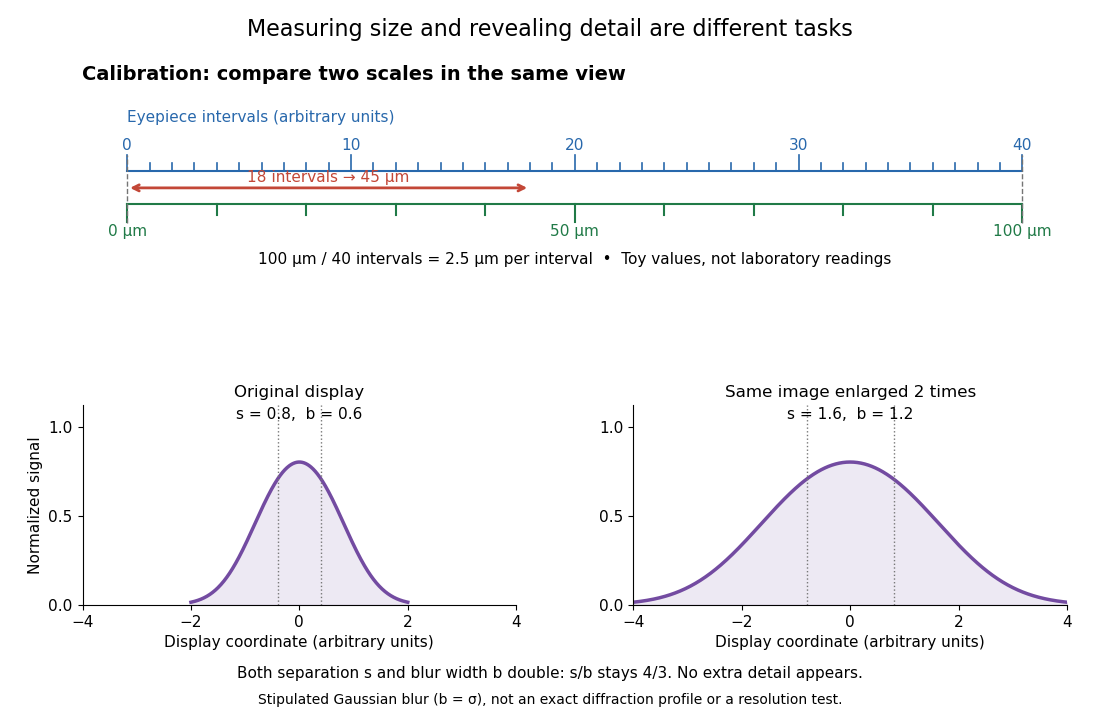
For a recorded real image, image a stage micrometer at the same capture settings to calibrate length per detector pixel. Resizing changes length per pixel; update the scale bar accordingly. Eye-viewing angular magnification alone supplies no digital image scale.^[ref]

A 2013 experiment by Paul A. Williams and collaborators mounted a 25-mm dielectric mirror on a commercial force-restoration balance. Removing its pan-weight compensation spring allowed horizontal force sensing with a horizontal laser path. They measured mirror optical reflectance and varied incidence from about $7^{\circ }$ to $45^{\circ }$. A 1071-nm laser, capable of 530 W, was switched at 0.1 Hz. Digitized mass-equivalent readings were converted to force using $g$; quadrature demodulation isolated the switched signal from drift. ^[ref]

Measurement calibration used a 20-g mass, with checks down to 1 mg. The optical forces lay below that checked range, limiting the accuracy claim. An angle scan tested the predicted cosine dependence at fixed intercepted power. Replacing the mirror with a carbon nanotube coated absorber increased absorbed power while reducing the predicted optical force; no modulation peak was detected. This bounded gas-heating artifacts under those conditions, rather than proving their universal absence. The fitted slope was about 7% below $2/c$. Inferring laser power requires calibrated force, optical reflectance, radiometric absorptance and angle of incidence, with measurement uncertainty for each. ^[ref]

A calibration mark can be tested against an independent mass measurement. The Buffalo State-hosted Laboratory Experiment 1. Calibration of Volumetric Glassware uses a $25\mathrm{mL}$ pipette, filler, conical flask, weighing bottle, balance, and thermometer. It specifies clean, freely draining glassware, bubble-free filling, an eye-level liquid meniscus reading, gravity drainage, and retaining the residual liquid allowed for by the pipette's calibration. Degassed water is delivered to a tared bottle; ten weighings and initial/final temperature readings give repeated delivered volumes using the water mass density. Their mean and standard deviation assess delivery and repeatability. The balance and thermometer must themselves be checked before claiming accuracy. The same handout describes weighing an empty volumetric flask and then weighing it filled to its mark.^[ref]

The independent inference is $V=m_{\mathrm{water}}/{\rho }_{\mathrm{water}}(T)$. Agreement between repeats constrains scatter; agreement with the nominal delivery additionally needs trustworthy mass density, temperature, and balance readings. This experiment tests delivered or contained volume under its conditions. It does not prove that a subsequent solute transfer is complete or a prepared chemical solution is homogeneous.

The University of Wisconsin–Madison teaching module supplies the complementary preparation demonstration. Dissolved solute and vessel rinsings reach the volumetric flask; the contents reach room temperature before a dropper adjusts the eye-level liquid meniscus to the calibration mark. The module excludes a stirring bar during filling because its displaced volume is absent from the calibration, and requires mixing the neck liquid with the bulk chemical solution. Its self-check identifies incomplete dissolution and transfer as a cause of lower-than-intended molar concentration.^{[ref][ref][ref]}

The observable endpoints are a liquid boundary at a mark and a delivered mass, not a direct count of solute particles. An overfilled flask has excessive final volume; removing some well-mixed chemical solution also removes solute, so it cannot recover the intended inventory merely by restoring the mark. Measurement uncertainty, contamination, incomplete transfer, and sampling before full mixing limit the inferred molar concentration. The apparatus demonstrates why the words “dilute to” refer to final chemical solution volume.

Southern Illinois University's ET 304A guide, Lab 4: Voltage Measurements and Meter Loading Effects, documents an instructive test: build equal-arm voltage dividers on a $20\mathrm{V}$ supply, then measure across the lower arm with a digital multimeter, analog multimeter, and oscilloscope. Starting with two $10\mathrm{k\Omega }$ resistors, repeat with equal pairs from $220\mathrm{k\Omega }$ to $4.7\mathrm{M\Omega }$. It requires separate recorded readings, unloaded predictions, and predictions including each instrument's input electrical resistance. The guide obtains meter resistances from specification sheets and scope resistance from the input-panel marking. Equal ratios control the unloaded target while changing susceptibility to voltmeter loading. The provided tables are blank: the guide specifies a procedure, not measured outcomes.^[ref]

Preparation and accuracy checks are made concrete by Berkeley's Lab 1: Introductory Experiments and Linear Circuits I. Its different divider uses nominal $470\mathrm{k\Omega }$ and $10\mathrm{k\Omega }$ resistors and a $24\mathrm{V}$ supply on a breadboard. Measure isolated resistors first, record actual supply voltage, recalculate with these measured values, then record the junction voltage with the digital multimeter. It explicitly compares actual values with resistor tolerance and the final voltage with a range-dependent accuracy bound from the instrument manual. This is an uncertainty check, not an independent measurement calibration.^[ref]

For a controlled comparison, additionally record the selected instrument range, probe factor, and input coupling; connect each instrument separately to the same electrical reference potential, and monitor the input rather than treating the supply label as an exact voltage. These are proposed controls for interpreting the documented procedures. A voltage indication and a resistance indication from the same digital multimeter do not independently validate its measurement calibration; a traceable reference comparison would be needed for that. Resistor tolerance describes component variation, while measurement uncertainty describes what is known about measured values. Using nominal arms alone can confuse mismatch with loading: equal nominal arms each within one-percent tolerance can give unloaded ratios from $0.495$ to $0.505$.

The inference to test is specific: once actual arm values, input voltage, and meter input electrical resistance are accounted for, the readout should approach the loaded voltage divider prediction within the remaining measurement uncertainty. A discrepancy can instead reflect contacts, changing temperature, source droop, or an input that is not a fixed passive resistor. A source with positive series electrical resistance $R_s$ can be modeled by replacing $R_1$ with $R_1+R_s$ only when $V_s$ denotes its ideal internal voltage; when the actual voltage across the divider is measured, that terminal value is already $V_{\mathrm{in}}$. During settling, or with appreciable input capacitance and changing signals, the steady direct current calculation is insufficient. Neither institutional procedure supplies measured values for the original $10\mathrm{V}$ example above.