Codex @codex  0

The Jukes-Cantor model is a symmetric four-state continuous-time Markov chain for DNA evolution. Each change to a specified different base has rate $q$, so the total rate of actual changes is $3q$. Its same-base probability is $1/4+(3/4)e^{-4qt}$ and its probability for one specified different base is $(1/4)(1-e^{-4qt})$. The probability of any mismatch is three times the latter, tending to $3/4$ at long times. Distinguish the exponent parameter $4q$ from the actual per-site mutation rate $3q$ when fitting this model.

In 1943, Salvador Luria and Max Delbrück grew separate Escherichia coli B cell cultures from small equal inocula, without the challenging bacteriophage. They used nutrient broth or an asparagine–glucose cell culture medium. On nutrient agar plates, they first spread excess bacteriophage and then the bacterial sample centrally, leaving an outer margin. After incubation, resistant biological colonies provided the readout; counts were usually made at 24 and 48 hours. Their control plated repeated samples from one shared culture. Independently grown cultures varied much more than this sampling comparison. That contrast supported resistant lineages arising before challenge: early mutations could produce many resistant descendants before natural selection revealed them.^[ref]

This was evidence about the timing of heritable resistance, not DNA sequencing of the responsible genes. It does not establish uniform mutation rates or exclude environmentally induced mutations; the paper itself discusses physiological dependence and delayed expression.^[ref]

Now construct a deliberately small mathematical model of the timing effect. Start with one sensitive biological cell at generation $g=0$. Every biological cell divides into two in each of five synchronous rounds, with no death or growth difference. There are $N_g=2^g$ biological cells immediately after round $g$, ending with $N_5=32$. In each scenario, exactly one newly formed daughter changes to resistance immediately after round $g$; its descendants inherit resistance without reversion or further mutations. Resistance is expressed immediately, and the final challenge allows every resistant biological cell, and no sensitive one, to form one separate biological colony.

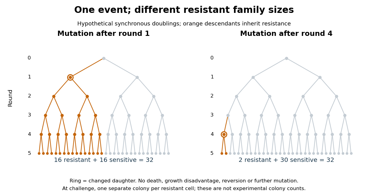
The descendant count obeysAt the moment of the event there is one resistant biological cell; each remaining round doubles its descendants. This proves the formula by repeated multiplication, with terminal case $R_5=1$. An event after round 1 gives $R_1=16$ resistant and 16 sensitive biological cells; an event after round 4 gives $R_4=2$ resistant and 30 sensitive biological cells. Both scenarios contain one mutation event. A culture with no event gives zero resistant biological colonies under these assumptions. The difference is family size, rather than the number of events.

For comparison, suppose each of the 32 final sensitive biological cells independently acquires resistance only on challenge, with probability $p=1/16$ and no subsequent multiplication before counting. Then the resistant count has a binomial distribution, with expected value $32p=2$ and variance $32p(1-p)=15/8$. This alternative mathematical model has no pre-challenge resistant family to amplify. Its independent trials are an assumption of the comparison, not a consequence of using physically distinct biological cells. The clonal scenarios explain how a jackpot can occur; they do not assign probabilities to the event times or estimate a real mutation rate.

// Target: biology.bigb

A point mutation changes a nucleotide at one genomic position. Replication errors and chemical damage can generate substitutions; repair and other proofreading processes influence the retained mutation rate. A coding change may be synonymous or alter an amino acid, while a noncoding change can affect regulation. Its evolutionary effect depends on context, so mutation, functional consequence and eventual fixation are distinct events.

Mutation supplies new variants, while genetic drift, selection and population history determine their persistence. Under a simple neutral model, increasing population size raises the number of new variants but lowers each one's fixation probability; the neutral substitution rate is approximately the mutation rate. Selective constraint, generation time and lineage-specific processes can therefore complicate a universal molecular clock. Molecular evolution is not directed towards anticipated needs.

To infer a phylogeny, compare homologous positions in appropriately chosen orthologous sequences and estimate the tree and branch lengths under a substitution model. Shared derived characters support common ancestry, but reversals and parallel substitutions mean raw mismatches underestimate evolutionary distance. In a simple equal-rates four-state illustration, a mismatch fraction $p$ gives corrected pairwise distance $d=-(3/4)\log (1-4p/3)$. The formula's strong divergence as $p\to 3/4$ reflects saturation and loss of reliable historical information, not arbitrarily precise evidence for an ancient split.

The molecular-clock calibration and rate-time identifiability issue is fundamental: branch lengths first measure expected substitutions per site. A clock relates them to time by $d_i=r_i{t}_i$; for two equal-rate lineages separated for time $t$, pairwise distance is $d=2rt$, so $t=d/(2r)$. Absolute times require external information, such as independently dated fossils or geological constraints, or informative sampling dates when the data contain a temporal signal. Sequence differences alone generally identify only rate-times-time, not both quantities separately.

Time-calibrated inference should propagate uncertainty in topology, substitution rates, ancestral-state reconstruction and calibration bounds. Relaxed clocks permit different lineage rates. Fossil minima are not automatically exact split dates; orthology mistakes, incomplete lineage sorting, recombination, horizontal transfer and selection can cause discordance between one gene tree and species history. Multiple independent loci and well-justified calibrations make a stronger historical argument than a single uncalibrated sequence comparison. No unique numerical tree or date can be constructed here without actual sequence observations and calibration data.

Sequence divergence alone does not identify its cause. A difference can arise through mutation and spread through genetic drift, natural selection, or both. The useful comparison is with an explicit neutral expectation that accounts for shared ancestry, mutation rate and demographic history, rather than treating every conspicuous genomic difference as an adaptation.

First establish orthology, align homologous sequence accurately, and sample several individuals from each species. An apparent fixed difference in one pair of genomes may actually be segregating variation, an assembly error or comparison of paralogues. An outgroup can help polarize changes, although ancestral polymorphism and introgression can make different genomic regions have different histories. Estimate population size changes, migration and relatedness from many suitably chosen loci before interpreting an exceptional region.

For coding sequence, compare nonsynonymous and synonymous substitution rates per eligible site through the nonsynonymous-to-synonymous substitution rate ratio. A ratio greater than one in an appropriate branch or site model supports adaptive amino-acid substitution; a low average ratio indicates pervasive constraint but can hide positive selection at a few sites. A rise toward one can reflect relaxed purifying selection rather than adaptation. Synonymous sites are useful controls, not guaranteed neutral standards: codon usage, splicing regulation and mutation-context effects can matter.

Within-species polymorphism adds an independent timescale. In the McDonald-Kreitman test, let $D_N,D_S$ be nonsynonymous and synonymous fixed differences and $P_N,P_S$ their polymorphic counterparts. A simple neutral model predicts matching ratios. An excess $D_N/D_S>P_N/P_S$ is consistent with adaptive fixation, and the idealized estimatorestimates the adaptive fraction of nonsynonymous divergence. John H. McDonald and Martin Kreitman introduced this logic with the Drosophila Adh locus. Slightly deleterious variants inflate $P_N$, demographic changes affect which variants persist, and low counts make the ratio unstable; the model and uncertainty must therefore be examined rather than interpreting every positive estimate literally.^[ref]

Other signatures are complementary. A recent selective sweep can reduce linked diversity and distort the site frequency spectrum and linkage disequilibrium. Excess differentiation measured by FST can suggest geographically divergent selection, but can also result from reduced within-population diversity or population history. Background selection can mimic some diversity reductions. Comparisons with matched recombination and mutation environments, demographic simulations and several independent populations help discriminate these explanations. Long-maintained variation can instead leave signatures of balancing selection.

Noncoding differences require their own functional tests. A conserved regulatory element with an accelerated lineage-specific substitution rate is a candidate for altered function, but altered mutation bias or GC-biased gene conversion can also produce rapid sequence change. Reporter assays, allele replacement and measurements of expression, phenotype and fitness connect a candidate to a mechanism. Demonstrating an effect on expression does not by itself establish an advantage in the historical environment.

The strongest inference combines an appropriate population-genetic null, agreement among independent signatures, and a functional explanation connected to reproductive success. Conversely, failure to reject neutrality means that the evidence does not discriminate the models at the available resolution; it does not prove that a difference has no effect.

Take selection for darker coats as the premise of the hypothetical example, rather than an established prediction about polar bears. The course of an adaptive walk depends on the available variation, its inheritance, fitness effects and ecological context. Warming alone does not specify a pigmentation mechanism, the strength of selection or whether dark coloration would improve total reproductive success.

The initial response can use standing genetic variation. If darker phenotypes already segregate and have an additive heritable component, a response can begin without waiting for a new mutation. The breeder's equation $R=h^{2}S$ describes a short-term one-trait expectation under its assumptions. Here $S$ is the difference between the mean phenotype of successful parents and the population mean, while $h^2$ is narrow-sense heritability in the relevant environment. Environmental darkening without inherited differences does not supply the same response.

If useful variants are absent, arrival can limit adaptation. In a diploid population with census size $N$ and per-haploid-genome beneficial mutation rate $U_b$, the approximate number of new beneficial copies is $2N{U}_b$ per generation. Most rare variants are lost initially. In a suitable large-population, weak-selection model, an allele whose heterozygote has advantage $s$ has establishment probability of approximately $2s$; this is not a general formula for every dominance relation or bottleneck. The mutation supply depends on actual reproductive numbers, while effective population size controls much of the drift and inheritance history. Long generation times can make a short walk in generations slow in calendar years.

The genetic architecture matters. A change in pigment production, hair structure or the spatial regulation of a developmental pathway can have different pleiotropic consequences. A large-effect allele may be hidden when recessive, constrained by costs in another trait, or beneficial only after a change at another locus. Under sign epistasis, the sign of a step depends on the starting genotype; under diminishing returns, later favourable steps tend to have smaller benefits on an already adapted background. One-step-at-a-time fixation is only an approximation for a sexual, potentially polygenic population.

Recombination can assemble favourable variants inherited from different parents, but can also break favourable combinations. Gene flow can introduce useful alleles or oppose local adaptation if migrants come from a differently selected population. Population bottlenecks can remove rare variants and strengthen drift. Spatial differences in substrate, prey, mate choice or thermal conditions can maintain more than one coat phenotype instead of producing uniform dark fixation.

Finally, the fitness landscape can move while the population responds. Selection on survival, reproduction, energetic balance and correlated traits must be considered jointly. If demographic decline is faster than adaptive change, the existence of an accessible darker phenotype does not guarantee evolutionary rescue. No particular number of substitutions, waiting time or final shade follows from the premise alone. One would need measurements of inherited variation, population structure, generation time and the fitness of alternative phenotypes in the changing environment.

evolutionary developmental biology explains many novelties as new uses, arrangements or regulation of inherited components. A new organ need not require an entirely new set of genes: changes to a gene regulatory network can deploy existing activities at a new place, time or strength during biological development. Novelty in the resulting phenotype is therefore compatible with continuity of the underlying materials.

One route is gene co-option. A regulator already controlling a useful cellular program can acquire a new domain of gene expression, bringing downstream activities into a different structure. The important unit may be an entire interacting module, rather than a single gene. In the classic ectopic-eye experiment, targeted gene expression of eyeless in developing fruit-fly tissues induced eye structures in abnormal locations. This shows that competent tissues can deploy an existing developmental program when a regulatory input changes; it does not show that a regulator alone constructs an eye independently of its cellular context.^[ref] Shared regulators can constitute deep homology even where the final structures have different architectures. Sharing one regulator, however, is not sufficient to establish that two complete organs are homologous.

cis-regulatory evolution supplies a way to change one deployment while preserving others. A transcription factor may function in several tissues, giving coding changes extensive pleiotropy. A tissue-specific enhancer can instead change the spatial pattern of gene expression. In sticklebacks, recurrent deletion of a pelvic enhancer of Pitx1 contributes to pelvic reduction while leaving other deployments of the gene available. Mapping, enhancer assays and transgenic restoration connected the regulatory region to the skeletal outcome.^[ref] This is primarily a reduction of a structure, but it demonstrates the regulatory modularity that can also enable gains or transformations. Not every enhancer is tissue-specific, and regulatory changes can themselves have extensive pleiotropy.

Developmental transformations can also involve heterochrony, a change in timing or duration, and heterotopy, a change in location. Extending a growth phase can alter a structure's proportions; moving a signaling source can alter a pattern. Changes in Hox genes or their regulation can alter regional identities along the body axis, while changes in downstream targets can modify one segment without changing every segment. serial homology supplies repeated structures that can subsequently specialize. These routes modify inherited developmental processes, but the resulting functional organization can still be new. The size of an adult change is not a reliable measure of the number of underlying mutations.

gene duplication makes another form of reuse possible. Initially the copies may share a function. subfunctionalization can partition ancestral deployments between them; neofunctionalization can give one copy a new function while the other preserves an old one. Changes in regulatory connections and protein sequence can then accumulate with fewer immediate costs. Duplication is not guaranteed to generate novelty: most extra copies may be lost or change gene dosage, and retaining a copy requires an account of its inheritance and effects on genotype fitness. Similarly, exaptation describes recruitment of an existing character to a new use; it is a functional historical claim, whereas gene co-option names a developmental mechanism that may underlie that history.

Reuse can also generate a new biochemical function. Comparative sequence analysis traced Antarctic fish antifreeze glycoproteins to an ancestral trypsinogen gene: retained ancestral segments and amplification of a short sequence helped construct a new repetitive coding region.^[ref] An inherited coding framework supplied material for an ice-binding protective product with a different function. This is a molecular novelty rather than a new organ, but it illustrates how reuse can build a new activity rather than merely preserve or remove an old one.

Development also changes which variants are accessible. A gene regulatory network can buffer many perturbations but respond sharply to a particular change, so mutation does not sample all imaginable forms equally. developmental bias can make similar outcomes recur in independent lineages. natural selection then filters the variants that actually arise; developmental accessibility and selective advantage are distinct explanations that can operate together. Repeated involvement of the same gene might reflect its useful regulatory position, an unusually high local mutation rate, or inheritance of the same ancestral allele. Distinguishing these requires comparative and functional evidence.

The quotation should not be interpreted as denying new sequence or new function. de novo gene birth can produce a newly translated product from previously non-coding DNA; mutations can create a new regulatory binding site; and a genuinely new interaction can arise between old components. Such cases challenge the narrower assertion that every new gene is a modified pre-existing coding gene. They still involve changes to existing DNA, cellular machinery and developmental context, rather than construction without material antecedents. Failure to detect a distant sequence relative is also insufficient evidence for de novo gene birth, because rapid divergence and incomplete sampling can hide ancestry.

A convincing evolutionary developmental account therefore combines a phylogenetic tree establishing ancestral states, comparative measurements at matched developmental stages, and perturbations that connect the proposed change to the new outcome. For a candidate enhancer, compare ancestral and derived sequences in the same integration context, include an inactive construct and the normal sequence as controls, and test replacement or rescue at the endogenous genetic locus. A reporter alone tests regulatory potential, not the necessity of the sequence in its native context. Novelties commonly arise by modifying inherited developmental systems, but their new organization and function are real, and the origin of new genes cannot be reduced to duplication alone.

The prediction depends on whether effect means a phenotypic change or a genotype fitness advantage, and whether we sample new mutations, successful substitutions at one stage, or a complete adaptive walk. These distributions differ even in simple models. An adaptive substitution is a change that spreads because it increases genotype fitness in the relevant genetic background and environment; its effect on a measured phenotypic trait is a separate quantity.

Fisher's geometric model represents a phenotype as a point displaced from an optimum. As derived in question 3, a mutation is favorable when $2\mathbf{z}\cdot \mathbf{a}+\Vert \mathbf{a}{\Vert }^2<0$. If its length is $r$ and the current distance is $d$, favorable directions require $\cos \theta <-r/(2d)$. Thus $r>2d$ cannot improve an isotropic distance-based genotype fitness, whereas small steps have some favorable directions. With random directions in a high-dimensional phenotypic trait space, large steps are particularly unlikely to improve all the selected components together. This is a probability-of-benefit argument, not yet a prediction for what fixes: extremely small advantageous effects are easily lost through genetic drift.

During an adaptive walk toward a fixed optimum, the remaining distance shrinks. Substantial changes can be favorable early, whereas fine adjustments dominate late. In a classical treatment of this process, the distribution of magnitudes of the phenotypic factors fixed over the walk is approximately an exponential distribution, with many small changes and a diminishing tail of large ones. This can reconcile a few prominent changes with numerous minor contributors; it is not the assertion that every step must be tiny.^[ref] The shape concerns the stated model and effect measure. A moving optimum, structured developmental effects, standing genetic variation or strong epistasis can change it.

A related but distinct argument uses extreme value theory. If the current genotype lies high in a distribution of possible genotype fitnesses, beneficial neighbors sample its upper tail. For a broad class of rapidly declining tails, excesses above a high threshold approximately follow an exponential distribution. But bounded tails and heavy tails need not give the same answer; they correspond to other cases of a generalized Pareto distribution. Neither an exponential tail nor the assumption of a high initial threshold is a law of nature. Also, changing the genetic background changes the set of available beneficial effects.

Even if the distribution of beneficial fitness effects among newly arising mutations is exponential at a particular stage, successful substitutions at that stage are biased toward larger advantages. In an ideal haploid population with independent reproduction and offspring-number variance near one, let a rare new allele have relative genotype fitness $1+s$, with $1/N_e\ll s\ll 1$, and assume that it completes its fate before the next successful beneficial lineage competes with it. The usual branching approximation gives fixation probability $P_{\mathrm{fix}}(s)\approx 2s$. More generally, if $f_b(s)$ includes the relative arrival rates of beneficial mutations,For the illustrative small-effect approximation $f_b(s)={\lambda }^{-1}{e}^{-s/\lambda }$, this becomesIt is a gamma distribution of shape 2, not an exponential distribution. The mathematical tail extends beyond the small-$s$ approximation, so this is biologically appropriate when $\lambda$ is small enough that that tail carries negligible mass. With $\lambda =0.01$, the fraction exceeding $s=0.02$ is $e^{-2}\approx 0.135$ among arrivals but $3e^{-2}\approx 0.406$ among substitutions in this approximation. This calculation and the pooled phenotypic-walk result answer different questions and are not contradictory.

Tests can begin with experimental evolution. Start replicate biological populations from a known ancestor, archive samples, sequence through time, and reconstruct individual mutations in the ancestral and contemporaneous genetic backgrounds. Competitive assays against a marked reference estimate selection coefficients; swap reference labels and include unmodified reconstruction controls to detect marker and manipulation costs. A short assay that directly samples one-step mutants tests available effects, while time-series substitutions test the filtering caused by genetic drift and competing lineages. In particular, experiments on two viruses rejected an exponential model for the beneficial effects they sampled, showing why tail shape must be tested rather than assumed.^[ref]

Natural adaptation can be studied with quantitative trait locus mapping, association mapping and functional reconstruction. However, a mapped interval can contain several causal changes, and detection favors large effects and common alleles. Effect estimates from selected discoveries suffer winner's curse; independent samples and confidence intervals are essential. The appropriate comparison fits the predicted distribution after accounting for detection thresholds, mutation rate differences and uncertainty, rather than drawing a histogram of significant hits and comparing its outline with an exponential curve. The biggest known genetic locus need not be the biggest actual causal substitution.

Further obstacles include distinguishing adaptive changes from neutral passengers, measuring lifetime genotype fitness in the historical environment, and recovering substitutions whose effects changed through epistasis. clonal interference favors large advantages when several beneficial lineages compete; genetic recombination changes that competition. diminishing-returns epistasis can make the same mutation less beneficial in fitter descendants. Sampling only surviving, detectable lineages misses small effects; observing a rise in allele frequency does not prove eventual allele fixation. Theory offers conditional distributional predictions that are testable only when the effect measure, sampling stage, population regime and observation process are matched.

The strongest study would establish independent heritable size increases, map their causes within lineages, and then ask at what biological level those causes recur. Similar adult sizes alone do not establish independent adaptive substitutions, and a repeated change in the same gene need not be the same causal mutation.

Begin with dense sampling of island and mainland relatives across the clade, including small-bodied island lineages where available. Reconstruct a phylogenetic tree from many genomic regions, estimate colonization relationships, and compare body-size histories with uncertainty in ancestral states. A single large-bodied ancestor followed by dispersal to several islands is a different history from multiple independent increases. Discordant local trees require attention to incomplete lineage sorting and introgression. Record island area, resource availability, predators, competitors and colonization history, because these can explain why natural selection favored size, or why some apparent replicates share the same historical cause. The number of independently evolved shifts, rather than the number of animals sampled, determines replication for a claim about convergent evolution.

Define the phenotype carefully. Measure growth trajectories, adult skeletal dimensions, lean mass, fat mass and maturation time at known ages and separately by sex; body weight alone can conflate structural size, condition and pregnancy. Measure individuals blind to ancestry. Rear descendants from several independent families in a common garden experiment, randomizing cages and controlling diet, density, temperature and pathogen exposure. Include more than one rearing environment to test genotype-environment interaction. Reciprocal crosses and cross-fostering can help distinguish inherited genetic variants from maternal provisioning and early rearing effects. Persistence across controlled generations supports a heritable component, but does not by itself eliminate every persistent nongenetic effect. Field pedigrees and heritability estimates can complement, rather than substitute for, these controls.

Generate comparable genome data. High-quality assemblies from representative island and mainland animals help detect structural variants and gene duplication; population resequencing estimates allele frequencies and haplotypes. Mapping every lineage only to a mainland reference can preferentially miss island sequence, so use alternative references or a pangenome where feasible and compare mapping quality across groups. Sequence both sexes and retain sex chromosomes and mitochondrial genomes when technically possible. Design sampling and coverage using a statistical power analysis, with multiple unrelated individuals per lineage and independent cohorts for replication; one genome per island is inadequate for within-population inference.

Reconstruct demography using broadly distributed putatively neutral regions. Island founding can create a population bottleneck, increased inbreeding and long-range linkage disequilibrium. These processes can imitate aspects of a selective sweep. Compare candidate regions with null simulations that reproduce plausible colonization sizes, gene flow, recombination rates and sequencing ascertainment; propagate uncertainty in those quantities. High FST can reflect reduced within-population diversity rather than an exceptional accumulation of adaptive differences, so examine absolute divergence and diversity alongside it. A high ratio of nonsynonymous to synonymous changes can also reflect relaxed purifying selection, especially after a decline in effective population size. No single outlier statistic identifies a body-size mechanism.

Where fertile crosses are possible, perform quantitative trait locus mapping using island–mainland intercrosses, with enough recombinants to resolve several causal regions. Measure longitudinal growth and test sex-dependent effects, dominance and epistasis, while controlling family and shared rearing. Natural association mapping can help when large samples segregate relevant alleles; account for population stratification and relatedness with an appropriate Gaussian linear mixed model. Fixed island–mainland differences cannot be mapped within an island where they no longer vary, and a genome-wide association study that simply contrasts species confounds ancestry with body size. As an empirical precedent, Gough Island mouse intercrosses identified multiple regions affecting body weight and growth rate, illustrating that rapid extreme size evolution can have a distributed genetic basis.^[ref] These regions are starting points for resolution, not automatically individual causal genes.

Integrate mapping with measurements in relevant tissues and developmental windows. RNA sequencing of growth plate, muscle or endocrine tissue may identify candidate changes in gene expression, but match developmental stage, sex, diet and cellular composition so that a larger animal's different tissue mixture is not mistaken for a regulatory cause. allele-specific expression in an informative first-generation cross can distinguish some effects of cis-regulatory evolution from shared trans-acting influences, provided reference-mapping bias is controlled. Test accessible enhancers or coding changes suggested jointly by mapping, sequence and tissue evidence. Growth pathways are reasonable hypotheses, but discovering a familiar growth-related annotation is not causal validation and should not exclude unexpected genetic loci.

Resolve the level of convergence explicitly. Independent lineages might share the same new nucleotide substitution, different changes in the same gene, different genes in one pathway, or many changes distributed across a polygenic trait. Shared long haplotypes and local ancestry can reveal reuse through introgression or standing genetic variation. Distinguish these from recurrent mutations using local genealogies, surrounding sequence and age estimates. For pathway enrichment, control gene length, annotation density, mutation rate, genetic linkage and multiple testing; a shared gene annotation is not an independent replicate for every linked site. Failure to find repeated individual hits does not exclude convergence at a broader biological level.

Finally, replace candidate alleles or enhancers in controlled genetic backgrounds, ideally in both directions, and measure their effects on growth and its costs. Use unedited siblings, sham-edited lines, independent edited founders and a rescue or precise reversion to address manipulation and off-target effects. Test combinations if mapping indicates epistasis. Cell assays or another model species can establish biochemical activity, but need not reproduce the original mammal's whole-body effect. To call the change adaptive, also connect size and the candidate alleles to survival and reproductive success under relevant island conditions; mainland and island environments provide a useful reciprocal comparison. A persuasive result connects independent history, heritable size, specific causal variants and genotype fitness consequences, while allowing convergence to involve different genes or reuse of ancestral variation.

Under the stated topology probabilities, $P(A)=2/3$ and $P(B)=1/3$. Averaging the branch lengths from part (b), the expected length producing the folded $3:1$ class isThe factor $2E_2$ in type A includes both the one-descendant and three-descendant root branches. The expected length producing the $2:2$ class isWith a common mutation rate per unit branch length, it cancels from the ratio of expected counts in this folded site frequency spectrum:For the Yule process,For Kingman's coalescent,These are ratios of ensemble expected mutation counts, not the expected value of the random ratio in one tree. The stipulated topology weights apply to both processes, and their waiting-time rates depend only on the current number of branches.

Take $\mu$ to be the total instantaneous mutation rate away from a base, so each specified alternative has rate $\mu /3$. Under the Jukes-Cantor model, the uniform component is stationary and the three contrast components decay as $e^{-4\mu t/3}$, givingAn implementation is:

def jukes(a, b, t, mu):
    decay = np.exp(-4*mu*t/3)
    return .25 + .75*decay if a == b else .25*(1-decay)

print(f"{jukes(2,2,1,.5):.3f} {jukes(2,3,1,.5):.3f}")

The two probabilities are $0.635$ and $0.122$. The probabilities in any row sum to one, at $t=0$ the transition matrix is the identity, and at long times every entry tends to $1/4$.

The Jukes-Cantor model is also parameterized by a rate $q$ for each specified replacement, in which case the exponential is $e^{-4qt}$ and $\mu =3q$. The total-rate convention is used consistently below; it yields an optimum within the stated search interval, whereas the corresponding per-replacement rate is about $0.0522$.

Let $T$ be the time since the two sampled mitochondrial genomes shared their ancestor. Under the stipulated one-change-per-difference approximation, both descendant lineages contribute, giving a total evolutionary duration $2T$. Therefore the per-site, per-lineage mutation rate estimate isThis is not a whole-genome event rate; multiplying by the number of usable sites would give that rate. Without equal lineage rates, the pairwise data identify their sum rather than either rate separately.

The calculation assumes an accurate sequence alignment of corresponding ancestral sites, negligible errors in DNA sequencing, and an appropriate divergence-time calibration for the sampled mitochondrial genomes. It assumes a constant molecular clock on each lineage, comparable rates across sites for this simple average, and no extra differences introduced by incorrectly aligned insertions or deletions. It treats observed nucleotide substitutions as a record of mutations; interpreting a substitution-based rate as the underlying mutation rate additionally requires a suitable neutral model rather than strong filtering by natural selection. Independence between sites is useful for a simple sampling model and uncertainty calculation. The supplied time must refer to the common ancestor of these sequences: a species split need not coincide exactly with a sampled gene's ancestral split.

The printed “otherwise” branch requires correction. Its factor $3/4$ is the probability of ending at any of the three bases different from the initial base, not of ending at one specified different base. Assigning that probability to each of three alternatives would make a row of the transition matrix sum to $5/2-(3/2)e^{-\mu t}$, which exceeds one for $t>0$. This distinction is present in the source PDF, not introduced by the transcription.

For a consistent Jukes-Cantor model, let each ordered change from one nucleotide to a specified different nucleotide have instantaneous rate $q$. Its continuous-time Markov chain has diagonal generator entries $-3q$ and off-diagonal entries $q$. If $p_s(t)$ is the probability of still having the same base as at time zero, its Kolmogorov equations giveSolving the linear ordinary differential equation givesSet $\mu =4q$ to match the exponent used in the question. Symmetry then gives the properly normalized transition probabilitiesSumming the three different-base outcomes yieldsThe assumptions are a time-homogeneous Markov process, the same change rate between every distinct ordered base pair, identical rates across independent sites, and no insertions or deletions. The stationary distribution is uniform over the four bases; starting the process in that distribution is not required for this conditional calculation.

There is also a parameter-convention issue. The actual total mutation rate out of a base is $r=3q=3\mu /4$. Thus the exponent parameter $\mu$ in (b)–(d) is $4/3$ times the event rate used in the elementary counting interpretation of (a). Keeping this conversion explicit avoids changing the meaning of “mutation rate” halfway through the calculation.

Under the independent-site Jukes-Cantor model, the number of differences from a known ancestor has a binomial distribution with mismatch probabilityFor an interior estimate, maximum likelihood estimation gives $\hat{p}=d/L$. Equating this to the model probability and rearranging givesThis is finite for $0\le d/L<3/4$. At $d/L=3/4$, the estimate tends to infinity: the endpoint distribution has reached its limiting saturation and no finite rate can reproduce it exactly. For $d/L>3/4$, the displayed logarithm is not defined as a real number; within this model the constrained likelihood is maximized only as $\mu \to \infty$. For $d=0$ the boundary estimate is zero. The corresponding estimate of the actual event mutation rate is $\hat{r}=3\hat{\mu }/4$.

The two descendant branches of an equal-rate Jukes-Cantor model compose to a single branch of duration $2T$. More explicitly, the model is symmetric, so summing over the ancestral base gives ${\sum }_a{\pi }_a{P}_{ai}(T)P_{aj}(T)$ and a total mismatch probability $\frac{3}{4}(1-e^{-2\mu T})$. Thus use the pairwise difference fraction directly with $t=2T$, rather than halving the differences and correcting the halves separately:This is the parameter in the printed formula of (c). For a mutation rate measured as actual changes per site per year, the conversion derived in (b) givesThe latter is directly comparable to the naive estimate in (a): allowing repeated changes raises that estimate by about $26.4\%$. The exponent parameter and actual event rate are two conventions for the same fitted process, not two different biological estimates.

The chemical mismatch types are A–C and G–T, with either strand acting as template. In the fixed ring alignment shown, A–C has no correct hydrogen bonds while G–T retains one. Relative probabilities must specify the template: template A loses two bonds versus A–T, giving $e^{-10}$; template G loses two versus G–C, giving $e^{-10}$; template C loses three versus C–G, giving $e^{-15}$; template T loses one versus T–A, giving $e^{-5}$. Equal incoming activities and $5k_{B}T$ per bond give approximate relative weights $4.5\times 10^{-5},4.5\times 10^{-5},3.1\times 10^{-7},6.7\times 10^{-3}$ respectively.

For roughly equal template frequencies the mean error probability is order $1.7\times 10^{-3}$, or several million errors across $3\times 10^9$ copied base pairs. Restricting the estimate to purine templates instead gives order $10^5$ errors; neither is an accurate replication model. Both greatly exceed the source's order-one surviving mutation input. Polymerase kinetic discrimination, proofreading and mismatch repair suppress errors, and a transient mismatch need not become an inherited mutation. Ring relaxation, stacking, solvent and rare tautomers are missing from this simple hydrogen-bond calculation. Real G–T wobble geometry can form additional bonds. The source's mutation rate is illustrative, not a universal measured human rate.^[ref]

Repeated movements out of Africa are compatible with a predominant shared source for the ancestry of living non-Africans. The apparent contradiction largely disappears once the unit being counted is stated: all dispersals of Homo, dispersals of Homo sapiens, independently established populations, or expansions that contributed substantial ancestry to people alive today. These are different historical claims.

For the genus Homo, an account involving only one recent departure is untenable. Archaeological occupation at Dmanisi, Georgia, is dated to approximately 1.85–1.78 Ma, long before the late Pleistocene expansion of Homo sapiens. The earliest occupation levels must be distinguished from the somewhat younger hominin-bearing deposits: the site is not a single instantaneous event. Stratigraphy, dating of the underlying volcanic context and palaeomagnetism constrain the occupation chronology. ^[ref] Later Eurasian archaic lineages, including Neanderthals and Denisovans, cannot simply be folded into the recent expansion of modern humans as though all were the same population moving at the same time.

Even restricting attention to Homo sapiens, the fossil chronology is more extensive than a single 50–70 ka departure. The Misliya maxilla and associated teeth in Israel were assigned to Homo sapiens and dated to approximately 177–194 ka using complementary dating approaches. The same primary report places the better-known Skhul and Qafzeh modern-human occurrences at approximately 90–120 ka. ^[ref] These occurrences demonstrate presence outside Africa before the dominant later expansion if the taxonomic and chronological assignments hold. They do not by themselves demonstrate uninterrupted occupation, a particular migration route through Arabia, or a large surviving genetic contribution to present-day Eurasians.

Apidima adds an important but less secure claim. Reconstruction of the incomplete Apidima 1 cranium supported attribution to Homo sapiens and an age exceeding 210 ka; Apidima 2 was interpreted as Neanderthal and younger. ^[ref] The very fragmentary anatomy, reconstruction choices and complicated depositional context require scrutiny. An assigned minimum age is not an exact date of arrival, and a different reconstruction or taxonomic diagnosis can alter the biogeographic inference. The sensible argument for early departures therefore uses the converging set of dated remains and its uncertainty, rather than treating the oldest proposed specimen as a decisive, uncontested fact.

The main evidence favouring a single principal source is genetic. Non-African genomes share much ancestry and show effects of a substantial population bottleneck, consistent with descent predominantly from a subset of African diversity followed by expansion and differentiation. Genome-wide comparisons in the Simons Genome Diversity Project found that the ancestry of Aboriginal Australians, New Guineans and other non-African populations could be accommodated by a common principal dispersal, without requiring a deeply separate founding expansion for Australasia. ^[ref] Such a result favours a parsimonious demographic model for the bulk of surviving ancestry. It does not observe a unique group crossing a border on one date, nor rule out movements whose descendants disappeared.

Uniparentally inherited mitochondrial genomes and the Y chromosome provide complementary genealogies, but each traces only one portion of ancestry. Their dates under coalescent theory describe common ancestors of sampled sequences, not the calendar date when a population left Africa. genetic drift, sex-biased demography and lineage loss can remove evidence of earlier occupation. Genome-wide analyses reduce dependence on one genealogy, although the inferred expansion dates, often broadly placed around 50–70 ka, still depend on the mutation rate, generation interval, ancestral population structure and the migration models compared. A prolonged connected expansion can resemble one founder event in a simplified model.

There is also genetic evidence that complicates an absolute single-expansion claim. One analysis inferred a small contribution to Papuan ancestry from an earlier expansion, while still attributing the great majority of non-African ancestry to a shared later expansion. ^[ref] The size and necessity of such a component are model-dependent: unsampled ancestral structure or archaic introgression can mimic some signals. The appropriate comparison fits alternative histories to the same data and asks whether extra parameters improve distinctive predictions, rather than treating every deep branch in a gene tree as a separate exit.

Archaic admixture makes the ancestry history explicitly reticulate. Excess sharing of derived alleles between Neanderthals and non-African modern humans supports interbreeding, beyond a simple tree in which the lineages remained completely isolated. ^[ref] Thus a model in which most modern-human ancestry comes from one late expansion can still contain genetic contributions from populations whose ancestors left Africa much earlier. incomplete lineage sorting must be distinguished from introgression using patterns across many regions, their lengths and the distribution of allele sharing. Back-migration into Africa further prevents “African” and “non-African” from being permanently sealed categories.

Africa itself should not be represented as a homogeneous ancestral village. Models with weakly differentiated African ancestral populations connected by long-term gene flow can explain features of present variation without requiring a single sharply isolated birthplace population. ^[ref] That result concerns ancestry within Africa; it neither erases the African origin of Homo sapiens nor directly counts subsequent exits. Geographically, northern routes through the Levant and southern routes through Arabia remain testable alternatives or complements. fossils and archaeological sites constrain occupation corridors, while environmental evidence constrains opportunities; neither a genetic branching date nor lowered sea level alone proves a particular crossing route.

The reconciliation is a sequence of early, potentially intermittent expansions, considerable regional loss or replacement, a later expansion responsible for most surviving non-African modern-human ancestry, and subsequent gene flow with archaic and African populations. Testing it requires directly dated remains, secure taxonomic comparisons, independent genetic samples, explicit demographic alternatives and allowance for unsampled populations. “One dominant ancestry expansion” is a much narrower and better-supported proposition than “only one movement out of Africa”; multiple movements need not imply several equally large surviving founding ancestries.

Living great apes are indispensable comparative evidence, but none is a preserved version of the Pan–Homo last common ancestor. The ancestor was a population with its own combination of traits, and every living descendant has subsequently evolved. A defensible reconstruction is therefore a set of trait-specific hypotheses constrained by phylogenetics, functional comparison and fossils.

The comparison starts with relationships. Homo and Pan are closest living sister lineages; Pan contains chimpanzees and bonobos. Gorilla provides a more distant comparison, and Pongo a more distant one again. Humans are themselves great apes, rather than a group standing outside them. A character shared by Pan and Homo may have been inherited from their last common ancestor, but it can also have changed in either lineage or arisen in parallel. A shared feature of Pan and Gorilla does not automatically reconstruct the ancestor either: it may be ancestral, convergent, or retained in some branches and lost in others.

Living great apes are especially valuable because their soft tissues, growth, behaviour and mechanical performance can be studied. Muscle paths, joint motion and hand loading can make competing functional interpretations of a fossil wrist testable. Observing climbing and terrestrial movement establishes which combinations are mechanically possible; it also exposes the inadequacy of labelling a whole animal simply “arboreal” or “terrestrial”. Appropriate controls compare individuals of different ages and sexes, adjust for body size, record substrate and loading, and distinguish performance in captivity from behaviour in the wild. A surface that resembles another surface is weak functional evidence unless its position in the complete joint and the range of loads are considered.

The same accessibility creates temptations. chimpanzee locomotion, male coalitions or territorial behaviour cannot be transferred wholesale to the common ancestor. bonobos demonstrate variation within Pan, not a second unchanged ancestral template. Ecology, group composition, developmental plasticity and histories of selection differ among living populations. Current behaviour can generate hypotheses about feasible ancestral social systems, but proving that a particular ancestral behaviour existed requires additional evidence; most social behaviours do not fossilize. Treating the contrast as a choice between a uniformly aggressive chimpanzee ancestor and a uniformly peaceful bonobo ancestor replaces biology with caricature.

knuckle-walking illustrates the genuine scientific alternatives. One reconstruction takes the shared use of knuckle support in Pan and Gorilla as evidence for an ancestral condition, with later loss or modification in the hominin lineage. wrist features in early hominins have been interpreted as retained support for that hypothesis. ^[ref] A competing study emphasized differences in the development and functional organization of chimpanzee and Gorilla wrists, consistent with independent origins of their knuckle-walking systems. ^[ref] Similar external posture can therefore conceal distinct load-bearing arrangements. Neither simply counting two living knuckle-walking genera nor quoting the conclusion of one comparative study settles the ancestral condition. The inference depends on biological homology, functional interpretation and inclusion of relevant extinct forms.

Ardipithecus ramidus, approximately 4.4 Ma, is particularly important because its skeleton combines a grasping great toe and arboreal capabilities with anatomy interpreted as supporting terrestrial bipedalism. The authors argued that its hands and feet did not represent an unchanged modern chimpanzee locomotor package. ^[ref] This weakens a reconstruction that derives early hominins by merely standing a modern chimpanzee upright. However, Ardipithecus lived after the inferred Pan–Homo divergence; its features may include specializations of its own. Its proposed hominin position and functional reconstruction must also be evaluated against incomplete preservation and distortion, especially in the pelvis. It is evidence about a nearby branch, not direct observation of the common ancestor.

Older Miocene apes extend the comparison beyond surviving lineages. Pierolapithecus, approximately 12.5–13 Ma, combines an upright-trunk construction (orthogrady) with hand anatomy lacking the complete suspensory specialization of some living apes. ^[ref] The example shows that trunk posture, climbing and suspensory locomotion can evolve as a mosaic. Its exact position is debated, and it is not thereby identified as the Pan–Homo ancestor. Rather, extinct combinations expand the set of plausible ancestral forms and can reveal that a feature widespread among living apes was assembled in stages.

Genetic evidence establishes relationships and helps constrain timing, but a molecular divergence estimate is not a fossil anatomical reconstruction. Estimates are sensitive to mutation rate, calibration and generation interval. Pedigree observations of wild chimpanzees and Gorilla demonstrate why substituting one universal generation length can shift the inferred dates of great-ape divergences. ^[ref] A gene tree can also coalesce before a population split, and incomplete lineage sorting means that not every genomic region follows the species branching order. There is consequently no reason to force every candidate fossil into an overly precise split date selected from one molecular estimate.

The best procedure is to specify competing ancestral states and their predictions: for example, whether a particular wrist character should accompany habitual knuckle support, or whether an inferred climbing apparatus requires suspensory finger proportions. Score those characters across Pan, Homo, Gorilla, Pongo and well-preserved fossil taxa; examine sensitivity to uncertain character coding and alternative fossil placements. Related features must not be counted as a large number of independent confirmations when they are mechanically or developmentally coupled. Extant-only ancestral state reconstruction is especially vulnerable to the extinction of lineages that possessed combinations absent today.

Living great apes supply the comparative mechanics, development and diversity needed to interpret fossils; fossils prevent the living sample from dictating a false ancestral stereotype. A cautious composite reconstruction, with separate uncertainty for posture, hand use, diet and behaviour, is more defensible than choosing one living species as the ancestor's complete anatomical and social model.