Past exam of the mathematics course of the University of Cambridge / 2014 / ib / Paper 1

The Steinitz exchange lemma says that if $u_1,\dots ,u_r$ are linearly independent and $v_1,\dots ,v_s$ span the same vector space, then $r\le s$ and, after reordering the $v_j$, the list $u_1,\dots ,u_r,v_{r+1},\dots ,v_s$ still spans it.

To prove this, suppose $u_1,\dots ,u_k$ have already replaced $k$ of the spanning vectors. Express $u_{k+1}$ in that spanning list. At least one coefficient of an unreplaced $v_j$ is nonzero: otherwise $u_{k+1}$ lies in the span of $u_1,\dots ,u_k$, contradicting linear independence. Solve this expression for that $v_j$ and replace it by $u_{k+1}$. The new list still spans. If all $s$ vectors were replaced before the $u_i$ were exhausted, the next $u_i$ would be dependent on its predecessors. Hence $r\le s$, and the replacement can continue through $u_r$.

For two bases of sizes $r,s$, apply the Steinitz exchange lemma in both directions to get $r\le s\le r$. Thus every basis has the same size. Given a linearly independent set and any finite basis, the replacement procedure produces a finite spanning list containing that set. Successively delete any remaining vector dependent on the others; none of the prescribed independent vectors need be deleted, since one can instead delete a dependent supplementary vector. Equivalently, greedily retain only supplementary vectors outside the span already built. The resulting list is a basis containing the prescribed set.

For the three-dimensional example, the columns have matrixTherefore the three vectors are a basis. For the four-dimensional example,This is a nontrivial linear dependence, so the four vectors are not a basis. The distinction is an instance of the adjacent sums of a cyclic basis criterion: alternating coefficients close consistently around an even cycle, but not an odd one.

Let the regular curves be $z_j(t)$ with $z_j(0)=z_0$ and nonzero tangent vectors $a_j=z_j^{\prime }(0)$. By the chain rule, their transformed tangents are $f^{\prime }(z_0)a_j$. Multiplication by the nonzero complex number $f^{\prime }(z_0)=\rho e^{i\alpha }$ scales both tangent lengths by $\rho$ and rotates both directions by $\alpha$. In particular,Thus the oriented angle, and hence the ordinary angle, is unchanged. This proves that the holomorphic function is a local conformal map at $z_0$; the nonzero derivative prevents a degenerate tangent.

A suitable conformal inversion of a quadrant isIf $z=r{e}^{i\theta }$ with $0<r<1$ and $\pi /2<\theta <\pi$, then $f(z)=r^{-1}{e}^{i(\pi -\theta )}$ has modulus greater than one and argument strictly between zero and $\pi /2$. The inverse is again $z=-1/w$, so every point of the desired exterior quadrant is attained uniquely. The origin is outside the open source region, and $f^{\prime }(z)=1/z^2\ne 0$ there.

Write $R=a+b\cos u>0$. The tangent vectors areTheir squared lengths and inner product give the first fundamental formThe unit normal determined by this ordered parametrization isTaking inner products of $\nu$ with ${\sigma }_{uu}$, ${\sigma }_{uv}$ and ${\sigma }_{vv}$ yields $e=b$, $f=0$, $g=R\cos u$. Consequently the second fundamental form of a ring torus isThis normal points into the tube. Choosing the outward unit normal reverses both coefficients and gives $-II$; the choice must therefore accompany an answer for the second fundamental form.

The Gaussian curvature is unchanged by that reversal:Since the denominator is positive, $K>0$ on the outside of the torus, where $\cos u>0$, and $K<0$ on its inner side, where $\cos u<0$. It vanishes on the two circles $u=\pi /2,3\pi /2$. This is the Gaussian curvature of a ring torus.

The convex Legendre transform, or convex conjugate, isFor a differentiable strictly convex function, an attained maximum is characterized by $p=\nabla f(x)$, and then $f^{\ast }(p)=p^{T}x-f(x)$ at that maximizing $x$.

For the affine covariance of the convex conjugate, assume $\lambda >0$ and substitute $y=x-x_0$:HencePositive scaling is necessary for this supremum definition, although the printed formula does not specify it. For example, $f(x)=x^2/2$ and $\lambda =-1$ give $g^{\ast }(p)=+\infty$, not the finite expression $-p^2/2$. If the transform is instead defined as a stationary value using a locally invertible gradient, the same algebraic identity holds for any $\lambda \ne 0$: the critical-point relation is $p=\lambda \nabla f(y)$, and substitution of that stationary $y$ gives the displayed formula. That extension does not assert a supremum for negative scaling.

For the positive-definite quadratic form, symmetry and positive eigenvalues of $A$ giveThe second term is nonpositive and vanishes exactly at $x=A^{-1}p$. Therefore

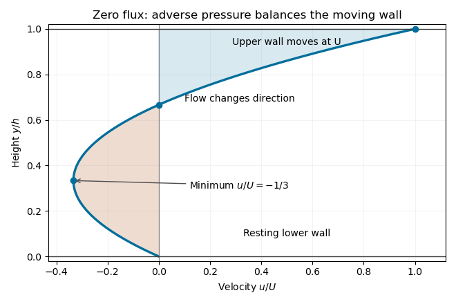
Take a steady parallel velocity $(u(y),0)$ and interpret the specified gradient as $p_x=G>0$. The horizontal Navier-Stokes equation reduces to $\mu u^{\prime \prime }=G$: the pressure force opposes positive $x$ motion. The no-slip boundary condition imposes $u(0)=0$, $u(h)=U$. Integrating twice givesThe velocity gradient is $u^{\prime }=G(y-h/2)/\mu +U/h$, an increasing function of $y$. It is negative somewhere in the channel exactly when its lower-wall limit is negative:Under this condition the negative-gradient interval is $0<y<h/2-\mu U/(Gh)$.

The volume flux per unit span isThus the zero-flux Couette-Poiseuille flow requiresThe profile starts at zero, reaches $u=-U/3$ at $y=h/3$, crosses zero at $y=2h/3$, and reaches $U$ at the moving wall. Negative and positive flux contributions cancel, even though the local velocity is nonzero.

Insert an exact smooth solution into the linear multistep method and define its unscaled local truncation error byIts Taylor expansion has coefficientsThe method has order at least $p$ exactly when $c_0=\cdots =c_p=0$, since then ${\mathcal{R}}_h[y]=O(h^{p+1})$ for every sufficiently smooth $y$. Necessity can be checked by inserting polynomials of successive degrees. This also corresponds to the usual truncation error ${\mathcal{R}}_h/h=O(h^p)$.

On the other hand, expansion of the characteristic polynomials of a linear multistep method givesThus the exponential-symbol order criterion for a multistep method isIf “order $p$” is meant to be the exact rather than guaranteed order, one additionally requires $c_{p+1}\ne 0$. The first two vanishing conditions are the usual consistency of a numerical method relations $\rho (1)=0$, ${\rho }^{\prime }(1)=\sigma (1)$.

The relevant one of the characteristic polynomials of a linear multistep method isThe coefficients on the right are chosen to give third order, so consistency of a numerical method is already available. By the Dahlquist equivalence theorem, convergence with convergent starting values is equivalent to zero-stability: every root of $\rho$ must satisfy $|w|\le 1$, and every root on the unit circle must be simple.

If $a<0$, the quadratic is negative at $w=-1$ and tends to $+\infty$ as $w\to -\infty$, so it has a root less than $-1$. If $a>1$, its root product is $a$, so at least one root has modulus greater than one. For $0\le a\le 1/4$, its real roots $(-1\pm \sqrt{1-4a})/2$ lie in $[-1,0]$. For $1/4<a\le 1$, its conjugate roots have modulus $\sqrt{a}\le 1$.

At $a=0$, the three roots are $1,0,-1$, with the unit-modulus roots simple. At $a=1$, they are $1,e^{2\pi i/3},e^{-2\pi i/3}$, again simple. The repeated quadratic root at $a=1/4$ is $-1/2$, strictly inside the unit circle, which the root condition for a multistep method permits. ThereforeThis is the root stability of a cubic multistep polynomial; oscillatory parasitic roots at the endpoints do not invalidate convergence when their starting amplitudes tend to zero.

For an estimator with finite second moment, its bias and mean squared error areWrite $\hat{\theta }-\theta =(\hat{\theta }-{\mathbb{E}}_{\theta }\hat{\theta })+b_{\theta }$. On squaring and taking expectations, the cross term vanishes. This proves the bias-variance decomposition of mean squared error:For the sample mean, independence gives $\mathbb{E}\bar{X}=\theta$, $\mathrm{Var}(\bar{X})={\theta }^2/n$. Thus $k\bar{X}$ has bias $(k-1)\theta$. Unbiasedness throughout the parameter family requiresAt the single parameter value $\theta =0$, all these estimators are zero almost surely; that special value does not change the requirement of unbiasedness for all $\theta$.

By the bias-variance decomposition of mean squared error,For $\theta \ne 0$, comparison with the unbiased estimator reduces toIts roots are $(n-1)/(n+1)$ and $1$, soEquality at either endpoint gives the same risk as $\bar{X}$. At $\theta =0$, every risk is zero, so no strict improvement is possible. This illustrates shrinking a sample mean with variance proportional to mean squared: allowing a small bias can reduce variance enough to improve total risk. The best constant is $k=n/(n+1)$, whose mean squared error is ${\theta }^2/(n+1)$.

A useful form of the Lagrangian sufficiency theorem is as follows. For minimization of $f(x)$ subject to $g_j(x)\ge 0$ and $h_i(x)=0$, formIf $x_{\ast }$ is feasible, ${\lambda }_j\ge 0$, ${\lambda }_j{g}_j(x_{\ast })=0$, and $x_{\ast }$ globally minimizes $L$ over the ambient domain for these fixed multipliers, then $x_{\ast }$ is a global constrained minimizer. Indeed, for every feasible $x$,The first inequality uses multiplier signs; the last equality uses feasibility and complementary slackness. Equality constraints alone require no sign restriction on their multipliers. A stationary point of a differentiable convex Lagrangian is a global minimum, which is a common way to verify the theorem's hypothesis.

Here takeStationarity gives $4x_1=4x_2=2x_3=\lambda$. Feasibility then gives $\lambda =1$ and $x_{\ast }=(1/4,1/4,1/2)$. For that multiplier,The Lagrangian has its unique global minimum at $x_{\ast }$, so the sufficiency theorem proves

If $x=0$, the generated subspace is zero and invariant. Otherwise, let $r$ be the first index for which $x,Tx,\dots ,T^{r}x$ are linearly dependent. Such an index exists with $1\le r\le n$, since there are $n+1$ vectors. The preceding vectors are independent, so the coefficient of $T^{r}x$ in this first relation cannot vanish. HenceThe linear operator $T$ sends each of the first $r-1$ generators to the next and sends the last into their span. This proves that their span is an invariant subspace. Every later iterate lies in the same subspace by induction, so it equals the span of the first $n$ iterates. Therefore the indicated subspace is $T$-invariant. This proof of a cyclic subspace uses only finite dimension and linear dependence.

The $n$ spanning vectors form a basis. WriteIn this cyclic basis the matrix is the companion matrixExpanding $\det (tI-C)$ along its last column givesFor example, the term containing $a_j$ has minor $t^j$ and the signs from the subdiagonal cancel the cofactor sign; the diagonal term supplies $t^n$. The defining relation says ${\chi }_T(T)x=0$. Every polynomial in $T$ commutes with $T$, soIt therefore vanishes on a basis, provingThis direct argument for a cyclic vector does not assume the Cayley-Hamilton theorem.

Since the first $k$ basis vectors span the invariant subspace $W$, their images have no components in the last $n-k$ coordinates. ThusHere $A$ is the matrix of $T{|}_W$, $D$ is the matrix of the induced map on the quotient vector space $V/W$, and $B$ is unrestricted. The chosen complementary span need not itself be invariant, so $D$ should not in general be called a restriction to that complement. The block-triangular determinant gives

Induct on $n$. The one-dimensional assertion is immediate, and the zero-dimensional case is vacuous. If $T$ has a cyclic vector spanning all of $V$, the direct proof in part (ii) applies. Otherwise choose $x\ne 0$ and let $W$ be its cyclic subspace. Part (i) makes $W$ invariant; the absence of a cyclic vector makes it proper and nonzero.

By induction, the restriction to $W$ is annihilated by ${\chi }_A$, and the induced map on $V/W$ is annihilated by ${\chi }_D$. The quotient assertion means ${\chi }_D(T)V\subset W$. Applying the restriction assertion next givesBy the characteristic factorization in part (iii), this is precisely ${\chi }_T(T)V=0$. HenceThis is the Cayley-Hamilton theorem from cyclic subspaces; using the quotient map is what makes the argument valid even when the block $B$ is nonzero.

If $|G|=p^{a}m$ with $p\nmid m$, a Sylow subgroup for $p$ is a subgroup of order $p^a$. The Sylow theorems assert: such subgroups exist; every $p$-subgroup is contained in a Sylow subgroup; all Sylow $p$-subgroups are conjugate; and their number $n_p$ divides $m$ and satisfies $n_p\equiv 1(\mathrm{mod}p)$.

For groups of order p squared q are not simple, if $p>q$, then $n_p\mid q$ and $n_p\equiv 1(\mathrm{mod}p)$ force $n_p=1$. Its unique Sylow subgroup is a nontrivial proper normal subgroup. Suppose instead $p<q$. If either Sylow count is one, the conclusion already follows. Otherwise $n_p=q$, while $n_q$ is either $p$ or $p^2$. The value $p$ is impossible because $0<p-1<q$. Thus $n_q=p^2$, and $q\mid (p^2-1)=(p-1)(p+1)$. Primality and $q>p$ imply $q\mid p+1$, hence $q=p+1$. The only consecutive primes are $p=2,q=3$.

In that exceptional order-$12$ case, four distinct Sylow $3$-subgroups contribute eight distinct nonidentity elements: their intersections are trivial. Only three nonidentity elements remain. Every subgroup of order four must contain exactly those remaining three, so there can be only one Sylow $2$-subgroup, contradicting the assumption that both counts were nontrivial. Therefore no group of order $p^{2}q$ with distinct primes is simple.

For the final factorization, normality of $H$ ensures $g^{-1}Pg$ is a Sylow $p$-subgroup of $H$. By Sylow conjugacy within $H$, choose $h\in H$ such that $g^{-1}Pg=h^{-1}Ph$. Then $k=g{h}^{-1}$ satisfiesThus $k\in N_G(P)$ and $g=kh$. We have proved the Frattini argumentThe normaliser factorization includes the case $P=\{1\}$, when its normalizer is all of $G$.

Two Lipschitz equivalent norms $N_1,N_2$ satisfy $c{N}_1(v)\le N_2(v)\le C{N}_1(v)$ for all $v$, for constants $0<c\le C<\infty$. These inequalities give the same convergent sequences in both norms. A subset of a metric space is closed exactly when it contains the limits of all convergent sequences from that subset. Therefore closedness is the same in the two norms.

For finite dimension, fix a basis $e_1,\dots ,e_d$ and let $x={\sum }_j{x}_j{e}_j$. For any norm $N$,The reverse triangle inequality then makes $N$ continuous in the Euclidean coordinate norm. If no positive lower bound existed on the Euclidean unit sphere, choose $x_m$ there with $N(x_m)\to 0$. By the Bolzano-Weierstrass theorem, a subsequence converges to $x$ on the unit sphere. Continuity would give $N(x)=0$, although $x\ne 0$, a contradiction. Thus $N$ is bounded below by a positive multiple of the Euclidean norm. Comparing any two norms through that coordinate norm proves all norms in finite dimension are Lipschitz equivalent.

On $C[0,1]$, nonnegativity, absolute homogeneity and the triangle inequality for $\Vert f{\Vert }_1={\int }_0^1|f|$ follow from the corresponding real-number properties and integration. If a continuous $f$ is nonzero at a point, it has absolute value bounded below by a positive constant on a nontrivial one-sided or two-sided interval around that point. Its integral is then positive. Hence $\Vert f{\Vert }_1=0$ implies $f=0$, completing the norm axioms.

For $n\ge 2$, put $g_n(x)=\max \{1-n|x-1/2|,0\}$ and $f_n=1-g_n$. Then $f_n(1/2)=0$, butThe limit function $1$ is not in the indicated point evaluation kernel. Consequently that set is not closed in the integral norm. This is the point-evaluation kernel is not closed in the integral norm phenomenon.

Finally $\Vert g_n{\Vert }_{\infty }=1$ while $\Vert g_n{\Vert }_1=1/n$. Thus no constant can bound the uniform norm by a multiple of the integral norm. Although $\Vert f{\Vert }_1\le \Vert f{\Vert }_{\infty }$ on this unit interval, the converse comparison fails: the two norms are not Lipschitz equivalent. The finite-dimensional theorem cannot be applied to this infinite-dimensional function space.

A compact space is one for which every open cover has a finite subcover. A Hausdorff space has disjoint open neighbourhoods of any two distinct points.

Let $K$ be a compact subspace of a Hausdorff space $X$, and let $x\notin K$. For each $y\in K$, choose disjoint open neighbourhoods $U_y$ of $y$ and $V_y$ of $x$. Finitely many $U_{y_1},\dots ,U_{y_m}$ cover $K$. Their corresponding intersection $V_{y_1}\cap \cdots \cap V_{y_m}$ is an open neighbourhood of $x$ disjoint from $K$. Thus $X\setminus K$ is open, proving compact subspaces of a Hausdorff space are closed.

In particular, $C_1\cap C_2$ is closed as a subspace of compact $C_1$. A closed subset of a compact space is compact: add its open complement to an open cover, apply compactness to the whole space, and discard that extra open set. Hence $C_1\cap C_2$ is compact.

In the cocountable topology on $\mathbb{R}$, two nonempty open sets always intersect. Their two countable complements have countable union, which cannot exhaust the uncountable real line. Therefore this space is not Hausdorff.

Every finite subset is compact in any topology. Conversely, from any infinite subset $C$ select distinct points $c_1,c_2,\dots$ and defineEach $U_n$ is cocountable and open; the sets increase and their union is all of $\mathbb{R}$. They therefore cover $C$, but a finite selection is contained in some $U_N$, which misses the infinitely many $c_j$ with $j\ge N$. No finite subcover exists. Thus the compact subsets of a cocountable space are

Use the positively oriented unit circle and $z=e^{i\theta }$. Writing $d=\sqrt{a^2-b^2}$, the contour integral for a sine-squared trigonometric quotient becomesThere is a double pole at zero and simple poles at $r_{\pm }=(-a\pm d)/b$. Since $a>b>0$, $|r_{+}|<1$ and $|r_{-}|>1$. The coefficient of $z^{-1}$ at zero is $a/(i{b}^2)$. At $r=r_{+}$, the residue isbecause $(r-r^{-1}{)}^2=4d^2/b^2$. The residue theorem consequently givesFor the second integral, use $x=\cos (\theta /2)$ with $0\le \theta \le \pi$. The square root is $\sin (\theta /2)$, and reversing the integration limits givesThe last factor uses the symmetry of the integrand about $\pi$ over a full period. Therefore

Substitute $y(x)={\sum }_{j\ge 0}{c}_j{x}^j$ into the Legendre differential equation. Matching the coefficient of $x^j$ givesChoose the parity of $n$: start with nonzero $c_0$ for even $n$, or nonzero $c_1$ for odd $n$, and set the other parity to zero. The numerator is nonzero for every preceding index of that parity below $n$, so $c_n\ne 0$, but at $j=n$ it vanishes. All higher coefficients are zero. This constructs a nonzero polynomial solution of degree exactly $n$.

Its value at $x=1$ cannot be zero. If it had a zero there of multiplicity $k\ge 1$, write $y=(x-1{)}^{k}R$ with $R(1)\ne 0$. The lowest-order term of $(1-x^2)y^{\prime \prime }-2x{y}^{\prime }$ would be $-2k^{2}R(1)(x-1{)}^{k-1}$, whereas $n(n+1)y$ starts at order $k$. The differential equation could not hold. Hence the polynomial can be scaled to satisfy $P_n(1)=1$.

The resulting Legendre polynomials beginEach satisfies both the differential equation and the specified normalization.

Set $U=R(r)\Theta (\theta )$ in the Laplace equation, multiply by $r^2/U$, and separate:Putting $x=\cos \theta$ turns the angular equation into the Legendre differential equation. For a solution smooth on the whole spherical axis, the allowed eigenvalues are $\lambda =n(n+1)$ with angular functions $P_n(\cos \theta )$. The radial equation has the two solutions $r^n,r^{-n-1}$. Superposition yields the regular axisymmetric expansionThe coefficients and convergence region are set by the domain and boundary data. Without regularity at the poles, singular Legendre functions and more general separated degrees would also be possible; they are excluded for this exterior spherical field.

The far-field matching fixes $A_1=v_0$ and all other growing coefficients to zero. The radial Neumann boundary condition at $r_0$ isIndependence of the angular modes gives $B_1=v_0{r}_0^3/2$ and all other decaying coefficients zero. Thus the exterior harmonic potential with no flux through a sphere isIts derivative vanishes on the sphere and its difference from $v_{0}r\cos \theta$ tends to zero at infinity. A spatial constant may be added if the far-field condition is intended only to specify the gradient or the leading growing term; matching the potential difference to zero fixes that constant to zero.

The squared sine has integral $a$ over the interval of length $2a$, since it contains an integer number of half-wavelengths. A real positive phase convention therefore givesInside the infinite square well, the Time-independent Schrodinger equation is $-{\hslash }^2{\psi }_n^{\prime \prime }/(2m)=E_n{\psi }_n$. The wavenumber is $\pi n/(2a)$, soThe stationary states vanish at both walls and form an orthonormal basis of the square-integrable state space. A common arbitrary phase on each basis function does not alter any energy or measurement probability.

Choose the prepared wavefunction real and positive on its support. Its normalization isIn the ramp-state expansion in a symmetric infinite well, write $\psi ={\sum }_{n\ge 1}{c}_n{\psi }_n$. Orthogonality givesFor $\kappa =n\pi /(2a)$, a primitive is $-x\cos (\kappa (x+a))/\kappa +\sin (\kappa (x+a))/{\kappa }^2$. Evaluating both endpoints givesAn equivalent parity-separated form isThese formulas with ${\sum }_n{c}_n{\psi }_n$ are the requested explicit expansion. The convergence is in the square-integrable norm; at the idealized discontinuity at the right wall, a pointwise boundary value does not change the quantum state or its probability amplitudes.

The original PDF threshold contains $\hslash$, not $h$. It is $8E_1$, so the energies strictly above it are exactly those with $n\ge 3$. By the Born rule, the required probability is $1-|c_1{|}^2-|c_2{|}^2$. The two excluded amplitudes areConsequentlyThus, in increasing powers of $1/\pi$,The threshold lies strictly between $E_2$ and $E_3$, so no equality-at-threshold convention affects the answer.

The Parseval identity for the orthonormal stationary-state expansion is ${\sum }_{n\ge 1}|c_n{|}^2=\Vert \psi {\Vert }^2=1$. Splitting the amplitudes into even and odd indices givesMultiply by ${\pi }^2/3$ to obtain the requested identity. Its integer constants areThe series converges absolutely, since both parity contributions are $O(p^{-2})$. This derivation uses the normalization of the prepared state and completeness of the well stationary states, rather than a separate summation trick.

An ideal conductor in electrostatic equilibrium has zero field in its interior and constant potential on its surface. Grounding fixes that potential to zero. The tangential field is continuous and therefore vanishes; the normal field has the jump fixed by the induced surface charge density $\sigma$:Here the normal points upward out of the conductor. The normal field is not generally zero; grounding prescribes the potential, not the induced charge density.