Past exam of the mathematics course of the University of Cambridge / 2019 / ib / Paper 2

Let $r=dim(U\cap W)$. Choose a basis $e_1,\dots ,e_r$ of the intersection of vector subspaces, extend it to a basis $e_1,\dots ,e_r,u_{r+1},\dots ,u_m$ of $U$, and independently extend it to a basis $e_1,\dots ,e_r,w_{r+1},\dots ,w_n$ of $W$. The combined listspans the sum of vector subspaces $U+W$. It is also linearly independent: a vanishing linear combination says that a combination of the $u_i$ belongs to $U\cap W$, and its expression in the chosen basis of $U$ forces all its coefficients to vanish; the coefficients of the $w_i$ then vanish in the same way. This proves the dimension formula for a sum of subspaces

Parametrize the two linear subspaces asPutting a vector of $U$ in $W$ first forces its fourth coordinate to vanish; the remaining defining equation is then automatic. Thusand the dimension formula gives $\dim (U+W)=2+2-1=3$.

The linear functionalvanishes on each displayed generator of $U$ and $W$. Its kernel is three-dimensional because $\ell \ne 0$, so the inclusion $U+W\subseteq \ker \ell$ between two three-dimensional subspaces is equality.

Let the torsion submodule of the module over a ring $M$ beThis is a submodule. Indeed, if $rm=0$ and $sn=0$ with $r,s\ne 0$, then $rs\ne 0$ because the scalar ring is an integral domain, and $rs(m+n)=0$; scalar multiples and additive inverses are handled similarly.

Take the quotient module $M_0=M/T(M)$ and let $q:M\to M_0$ be the quotient R-module homomorphism. It is torsion-free: if $0\ne r\in R$ and $r(m+T(M))=0$, then $rm\in T(M)$, so $srm=0$ for some $s\ne 0$. Since $sr\ne 0$, this puts $m$ in $T(M)$ and therefore $m+T(M)=0$.

Now let $N$ be torsion-free and let $f:M\to N$ be an $R$-module homomorphism. If $m\in T(M)$ and $rm=0$ for $r\ne 0$, then $rf(m)=f(rm)=0$, so torsion-freeness gives $f(m)=0$. Hence $T(M)\subseteq \ker f$, and the universal property of a quotient module gives a unique homomorphismwith $\boxed{f=f_0\circ q}$. Thus $M/T(M)$ is the maximal torsion-free quotient of $M$.

For $x\ne 0$, all component functions are continuously differentiable and the Jacobian matrix isAt a point $(0,y_0)$, the first component cannot be differentiable: along the first coordinate axis its difference quotient contains $h^{1/3}/h=h^{-2/3}$, which is unbounded as $h\to 0$. Therefore $f$ is continuously differentiable exactly at the points with $x\ne 0$.

At a point with $xy\ne 0$, the determinant of the derivative isThe inverse function theorem therefore supplies neighbourhoods on which $f$ has a continuously differentiable, hence differentiable, inverse. Concretely, if $(u,v)=f(x,y)$, the local inverse is the restriction ofwhich is continuously differentiable near the image whenever $y\ne 0$.

Suppose for contradiction that the continuous image of a connected space $Y=f(X)$ is disconnected. Then there are disjoint nonempty sets $U,V$, open in the subspace topology on $Y$, with $Y=U\cup V$. By continuity, $f^{-1}(U)$ and $f^{-1}(V)$ are disjoint open subsets of $X$; by surjectivity both are nonempty, and their union is $X$. This is a separation of a topological space of $X$, contradicting that $X$ is a connected space. Hence $Y$ is connected.

First recall from the least-upper-bound property that every real interval is connected. For completeness, if $[a,b]=U\cup V$ were a separation with $a\in U$, let $s$ be the supremum of the points $t$ for which $[a,t]$ remains in $U$. Relative openness rules out both $s\in U$ and $s\in V$: in the first case one can move slightly to the right while staying in $U$, and in the second one finds points of $V$ slightly to the left of $s$, contrary to the definition of $s$. Thus no separation exists.

Part (a) now makes $g([0,1])$ a connected subset of the real line. Such a set is an interval: if it contained $u<v$ but omitted $y\in (u,v)$, its intersections with $(-\infty ,y)$ and $(y,\infty )$ would separate it. Since $g([0,1])$ contains $g(0)$ and $g(1)$, it consequently contains every number between them. Therefore for each such $y$ there is an $x\in [0,1]$ with $\boxed{g(x)=y}$. This derives the intermediate value theorem from connectedness.

For an axisymmetric separated solution of the Laplace equation whose angular factor is the Legendre polynomial $P_n(\cos \theta )$, the radial ordinary differential equation has the two powers $r^n$ and $r^{-n-1}$. Thusfor constants $A,B$.

Write $x=\cos \theta$. Since $3\cos (2\theta )=6x^2-3=4P_2(x)-P_0(x)$, only the spherical harmonics of degrees zero and two occur. The degree-zero radial coefficient satisfying its two Dirichlet boundary conditions is $1-2/r$. For degree two, write $C{r}^2+D{r}^{-3}$; thenso $C=-4/31$ and $D=128/31$. By linearity and uniqueness of this boundary value problem,Direct substitution at $r=1,2$ verifies both boundary values.

The free-space Green function of the Laplacian for the Poisson equation gives the electric potentialFor $r=|\mathbf{x}|\gg R$, its electric multipole expansion begins withDefine the total electric charge and electric dipole moment byThen

The analogous solution for the magnetic vector potential isIts apparent $r^{-1}$ coefficient is ${\mu }_0(4\pi {)}^{-1}\int \mathbf{J}{d}^3{x}^{\prime }$. For each component, the supplied identity and the divergence-free vector field condition giveThe divergence theorem turns this into a surface integral outside the compact support of the current density, where $\mathbf{J}=0$. Hence $\int \mathbf{J}{d}^3{x}^{\prime }=0$, so the $1/r$ term vanishes.

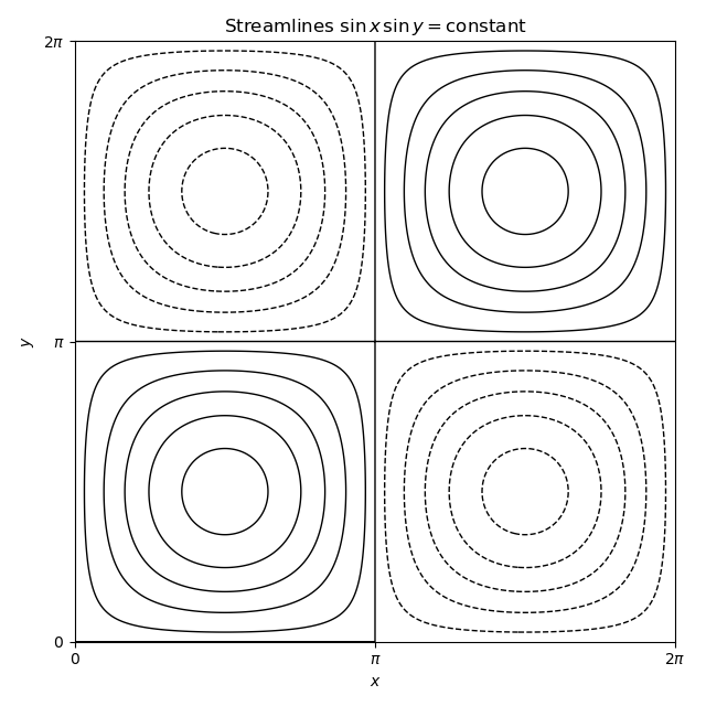
The velocity field is incompressible becauseWith the convention $u_x={\psi }_y$ and $u_y=-{\psi }_x$, a stream function isThe vorticity is vertical:For a steady inviscid incompressible flow, the vorticity equation is $(\mathbf{u}\cdot \nabla )\mathbf{\omega }=(\mathbf{\omega }\cdot \nabla )\mathbf{u}$. Here the right side is zero because the flow is independent of $z$, while the left side is $2(\mathbf{u}\cdot \nabla \psi ){\mathbf{e}}_z=0$ because velocity is tangent to the level sets of $\psi$. Thus the equation is satisfied.

The streamlines are the level curves $\sin x\sin y=\text{constant}$. The lines $x=\pi$ and $y=\pi$, together with the boundary, are separatrices; each of the four cells contains closed nested curves around a centre at $(\pi /2,\pi /2)$, $(3\pi /2,\pi /2)$, $(\pi /2,3\pi /2)$, or $(3\pi /2,3\pi /2)$.

Let $S={\sum }_{i=1}^n{X}_i$ be the number of heads. The likelihood function for the Bernoulli distribution sample is proportional to ${\theta }^S(1-\theta {)}^{n-S}$. A uniform distribution prior on $[0,1]$ is the $\mathrm{Beta}(1,1)$ distribution, so Beta-binomial conjugacy gives the posterior distribution

The quadratic loss, also called squared-error loss, for reporting an action $a$ when the parameter is $\theta$ is

For any action $a$, decompose the posterior expected quadratic loss around the posterior mean:The unique minimizer is therefore the Bayes estimator under squared error loss. Using the mean of the posterior Beta distribution givesUnder repeated sampling at parameter value $\theta$, $S$ has the binomial distribution with expected value $n\theta$. Consequentlyso its bias of an estimator is $(1-2\theta )/(n+2)$.

The Lagrange sufficiency theorem for maximizing $f$ subject to $g_i\ge 0$ and $h_j=0$ states that if a feasible point $x^{\ast }$ and multipliers ${\lambda }_i\ge 0,{\mu }_j$ satisfy complementary slackness and $x^{\ast }$ globally maximizes the Lagrangian function in constrained optimizationthen $x^{\ast }$ globally maximizes $f$ on the feasible set.

For the equality constraint, takeThe Lagrange multiplier equations giveso positivity and the constraint implyFor this multiplier, $L$ is a strictly concave function on the positive octant and its stationary point is its unique global maximum. The sufficiency theorem therefore proves that the constrained maximum is

For $x^2+y^2+z^2\le 1$, use $g=1-x^2-y^2-z^2$. The same point and multiplier satisfy feasibility, stationarity, $\lambda \ge 0$, and complementary slackness, and they again globally maximize the Lagrangian. Hence the answer is unchanged. Equivalently, any point with strict inequality can be radially scaled outward, increasing all three positive coordinates and therefore increasing $\log (xyz)$.

If $A$ is an invertible matrix, thenThus $AB$ and $BA$ are similar matrices, and similar matrices have the same characteristic polynomial.

For all but finitely many $s\in \mathbb{C}$, the matrix $A-sI$ is invertible. Part (a), applied to $A-sI$ and $B$, then givesBoth sides are polynomials in the two variables $s,t$. Since they agree for infinitely many values of $s$, their coefficients as polynomials in $s$ agree. Setting $s=0$ yieldseven when $A$ is singular.

TakeThen $AB=B\ne 0$ and $(AB{)}^2=0$, whereas $BA=0$. Hence their minimal polynomials are

For every nonnegative integer $k$,Consequently, if $m_{AB}(AB)=0$, thenBy the divisibility characterization of the minimal polynomial,Interchanging $A$ and $B$ also gives $m_{AB}(t)\mid t,m_{BA}(t)$. Therefore the Minimal polynomials of AB and BA can differ only in the exponent of the factor $t$, and that exponent differs by at most one.

If $AB$ is diagonalizable, its minimal polynomial has no repeated roots. The preceding divisibility says that every nonzero Jordan block of $BA$ has size one and every zero-eigenvalue block has size at most two. Squaring $BA$ preserves the one-dimensional nonzero blocks and sends every size-at-most-two nilpotent block to zero. Thus the Jordan normal form of $(BA{)}^2$ is diagonal, so

Because $f$ is irreducible, the ideal $(f)$ is maximal in the polynomial ring $k[X]$. Henceis a field extension of $k$. Let $\alpha =X+(f)\in F$. Evaluation in the quotient gives $f(\alpha )=0$, and the factor theorem in $F[X]$ givesfor some $g\in F[X]$. This is the standard adjoining a root of an irreducible polynomial construction.

Proceed by induction on $d=\mathrm{deg}f$. A nonconstant polynomial over a field has an irreducible factor $h$. Part (a) gives an extension $k_1/k$ containing a root ${\alpha }_1$ of $h$, hence of $f$. The factor theorem giveswhere $f_1$ is monic of degree $d-1$. Apply the induction hypothesis over $k_1$ and compose the resulting field extensions. The final field $F$ contains roots ${\alpha }_1,\dots ,{\alpha }_d$ andEquivalently, every polynomial has a splitting field.

Put $q=p^n$. Every extension of $k={\mathbb{F}}_p$ has characteristic $p$, so the iterated Frobenius endomorphism satisfiesThe root set is $K=\{a\in F:a^q=a\}$. It contains $0$ and $1$. If $a,b\in K$, thenso it is closed under subtraction and multiplication. If $a\in K$ is nonzero, thenThus $K$ is closed under multiplicative inverses as well, and is therefore a field. This is the polynomial characterization of a finite field; in fact it is the finite field with $q$ elements, since $X^q-X$ has degree $q$ and no repeated roots.

Two norms $\Vert \cdot \Vert$ and $\Vert \cdot {\Vert }^{\prime }$ on one vector space are Lipschitz equivalent when constants $c,C>0$ exist such that

Choose a basis of the finite-dimensional vector space and let $|x{|}_{\infty }$ be the maximum absolute coordinate. For any norm $N$, the triangle inequality givesso $N$ is continuous in the coordinate topology. On the compact set $\{x:|x{|}_{\infty }=1\}$, the positive continuous function $N$ attains a positive minimum $m$ and a finite maximum $M$. By absolute homogeneity,This proves the equivalence of norms in finite dimensions: every norm is equivalent to the maximum norm, and transitivity of these inequalities proves that any two norms on a finite-dimensional vector space are Lipschitz equivalent.

SupposeIf $(v_n)$ is a Cauchy sequence in $\Vert \cdot \Vert$, thenConversely, $\Vert v_n-v_m\Vert \le c^{-1}\Vert v_n-v_m{\Vert }^{\prime }\to 0$. Hence the sequence is Cauchy for one norm exactly when it is Cauchy for the other.

For each positive integer $N$, let $x^{(N)}$ have its first $N$ coordinates equal to one and all later coordinates zero. This is an element of the l-p sequence space for every finite $p$, andNo constant can bound $\Vert x{\Vert }_p$ by a fixed multiple of $\Vert x{\Vert }_{\infty }$ for all $N$. Thus $\Vert \cdot {\Vert }_p$ and $\Vert \cdot {\Vert }_{\infty }$ are not Lipschitz equivalent.

For $1\le p<q<\infty$, the same finitely supported sequence givesOne of the two inequalities required for equivalent norms therefore fails. Hence

Let $v_1,v_2\ne 0$ be tangent vectors to the two smooth curves at $p$. complex differentiability at a point givesWhen $f^{\prime }(p)\ne 0$, its real derivative is multiplication by a nonzero complex number, which is a rotation followed by a positive scaling. It therefore preserves the angle between $v_1$ and $v_2$, so $f$ is conformal at $p$. The condition is essential: $f(z)=z^2$ has $f^{\prime }(0)=0$ and sends rays making angle $\pi /4$ at zero to rays making angle $\pi /2$.

For $J(z)=z+z^{-1}$,If $z,w$ both satisfy $|z|>1$, or both satisfy $0<|z|<1$, the alternative $zw=1$ is impossible unless the points lie on the omitted unit circle. Hence $J$ is one-to-one on each region. Also $J^{\prime }(z)=1-z^{-2}$ has no zero there, so the restrictions are conformal. Solving $z^2-wz+1=0$ shows that $w\in [-2,2]$ exactly when both roots lie on the unit circle; otherwise one root is inside and the other outside. Thus each region has image

Taking the reciprocal of the interior restriction and filling its removable value at zero givesThe reciprocal sends $\mathbb{C}\setminus [-2,2]$ ontoand $g(0)=0$. Therefore $g$ is the required one-to-one conformal map from the unit disc.

A smooth surface in ${\mathbb{R}}^3$ is a subset locally parametrized by a smooth map of two variables whose derivative has rank two and which is a homeomorphism onto its image.

Writing $\rho =\sqrt{x^2+y^2}$, the first surface equation becomesIt is the torus of major radius $R=2\sqrt{2}$ and minor radius $r=1$, with smooth parametrizationSince $R>r$, this is an embedding. The Gaussian curvature of a torus is

For the second surface, use the orthogonal transformationIts equation becomes the same torus equation $(\sqrt{X^2+Y^2}-2\sqrt{2}{)}^2+Z^2=1$. Orthogonal transformations are Euclidean isometries and preserve Gaussian curvature. Curvature vanishes where $\cos v=0$, equivalently $Z=\pm 1$. In the original coordinates the zero-curvature points are therefore exactly

The two Euler-Lagrange equations areDifferentiating $\kappa =f-u^{\prime }{f}_{u^{\prime }}-w^{\prime }{f}_{w^{\prime }}$ along an extremal and using these equations gives $d\kappa /dx=f_x$. Hence the Beltrami identity makes $\kappa$ constant when $f$ has no explicit dependence on $x$. If $f$ omits $u$ or $w$, that variable is a cyclic coordinate and the corresponding momentum $f_{u^{\prime }}$ or $f_{w^{\prime }}$ is an additional first integral; continuous symmetries give the analogous conserved quantities through Noether's theorem.

Put $A=1-m/u$. Since $w$ is cyclic,for a constant $\lambda$. The Beltrami integral isTherefore

If $\kappa =-{\lambda }^2$, then $u^{\prime 2}={\lambda }^{2}m/u$ andFor $z>1$, definethe hinted identity gives $F^{\prime }(z)=z^{3/2}/(z-1)$. Hence $w=C\pm mF(u/m)$. Because $F(z)\to +\infty$ as $z\to \infty$, the prescribed limit selects the minus sign:As $u\downarrow m$, the logarithm tends to $-\infty$, so every such solution satisfies $\boxed{w\to +\infty }$.

Multiply the Gegenbauer differential equation byIt becomes the Sturm-Liouville formFor two polynomial solutions of degrees $m\ne n$, multiply their equations crosswise, subtract, and integrate over $(-1,1)$. The boundary term vanishes because $\alpha >0$ and $(1-x^2{)}^{\alpha +1/2}\to 0$. Since the eigenvalues $n(n+2\alpha )$ are distinct,Thus $a=-1$, $b=1$, and the displayed function is the weight.

Every interior root is simple: a solution and its derivative cannot both vanish at an ordinary point of a second-order linear differential equation unless the solution is identically zero. Let $x_1,\dots ,x_k$ be all interior roots and put $q(x)={\prod }_i(x-x_i)$. If $k<n$, then $q$ has degree below $n$, so orthogonality givesBut $C_n^{\alpha }/q$ has no zero and constant sign on $(-1,1)$, whence the integrand $q(x{)}^2(C_n^{\alpha }(x)/q(x))w(x)$ has one strict sign except at finitely many points. Its integral cannot vanish, a contradiction. Therefore $k=n$: all $n$ roots are real, simple, and lie in $(-1,1)$.

The total angular momentum operator isUsing the cyclic orbital angular momentum commutation relations,while $[L_z,L_z^2]=0$; hence $\boxed{[L_z,{\mathbf{L}}^2]=0}$. In Cartesian coordinates,Because $L_z(x+iy)=\hslash (x+iy)$ and it annihilates $z$ and every radial function,Replacing $i$ by $-i$ gives eigenvalue $-m\hslash$.

The six-dimensional space splits into the five trace-free quadratic spherical harmonics with $\ell =2$ and one radial state with $\ell =0$. A simultaneous eigenbasis for $L_z$ and ${\mathbf{L}}^2$ iswhere the eigenvalue $\ell (\ell +1){\hslash }^2$ of ${\mathbf{L}}^2$ was used. Every displayed state is a complex linear combination of the original six energy eigenstates, so it is still an energy eigenstate at the same level.

For a moving circuit, Faraday's law states that the electromotive forceequals $-d{\Phi }_B/dt$, where ${\Phi }_B={\int }_S\mathbf{B}\cdot d\mathbf{S}$ is the magnetic flux through any spanning surface. Choose the upward normal. The horizontal square hasso Ohm's law gives the induced currentwith positive current taken counterclockwise from above.

On the edge $x=a$, $d\mathbf{\ell }=dy{\mathbf{e}}_y$. The magnetic force on a current-carrying wire is $d\mathbf{F}=I,d\mathbf{\ell }\times \mathbf{B}$, henceThe ratio of the horizontal to vertical magnitudes is $2|z|/a$, so the directed force makes angle ${\tan }^{-1}(2z/a)$ with the vertical, with the sign fixing the horizontal side.

The horizontal forces on opposite edges cancel, while all four vertical contributions add:This is an electromagnetic drag force opposing the motion, as required by Lenz's law. Including gravity givesAt the terminal velocity, $\ddot{z}=0$, and the constant downward speed has magnitude