The coordinate tangent vectors are the partial derivatives of the position vector:Their pairwise dot products vanish. Their lengths, the scale factors of orthogonal coordinates, are . Since , the last is positive throughout the body. Thus these circular torus coordinates are orthogonal wherever ; at the cross-section angle degenerates, as in ordinary polar coordinates.
The ordered Jacobian determinant isIts sign is positive for , so the volume element is . The coordinate degeneracy on the central circle has zero volume and does not obstruct volume integration.
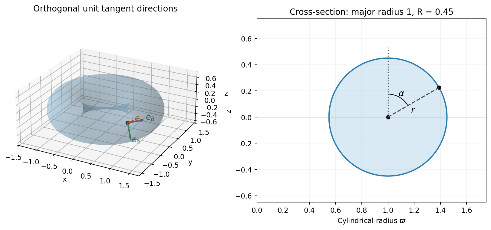
Circular torus coordinates and their orthogonal tangent directions
. Details. Take the closed surface with its outward orientation. For sufficiently smooth fields defined throughout the solid, the divergence theorem and the identity that the divergence of a curl is zero giveThus the curl term carries no net outward flux, and is independent of . The hole in the solid torus does not invalidate the divergence theorem; singularities of inside the integration region would invalidate the smoothness argument and must be excluded.
Only the quartic term contributes to the Laplacian. The mixed cubic has zero second derivative in each coordinate, while the exponential–trigonometric pairs are harmonic:Using and the Jacobian determinant from part (a), the divergence theorem givesThe term containing integrates to zero. Equivalently, the second vertical moment of a solid ring torus with major radius one is .
Remove the first spatial derivative by the Dirichlet gauge transform for constant drift:The nonzero exponential factor preserves the zero side and top values; it also preserves on the bottom. A separated product has the spatial eigenvalue problemsThe nontrivial solutions are for and for . There is no zero spatial mode in either direction. The temporal equation gives , whereTherefore the mixed-boundary drift-diffusion eigenmodes on a rectangle giveAt the temporal factors are one, giving the required expansion. The sine and mixed-end cosine bases are complete and orthogonal for . In particular,The factor four comes from the product of the two squared basis norms, each .
After multiplying the initial field by , the dependence is exactly the cosine mode. Its orthogonality therefore gives when . For , the remaining Fourier coefficient in the Fourier sine series isThusThe coefficients are independent of , because the initial exponential exactly cancels the drift-removing weight. Substitution into the preceding expansion gives the full subsequent solution, with decay rates .
For the Green function of , the homogeneous solutions satisfying the left and right endpoint conditions are and . Their Wronskian isContinuity of the kernel at and integration of require . Hence the Dirichlet modified Helmholtz Green function on an interval isHere and . The negative sign is essential for this operator convention. Integrating the forcing against the kernel givesThis satisfies both endpoint conditions. It solves the equation classically for continuous , and in the corresponding weak sense for integrable forcing. A homogeneous difference satisfying both endpoint conditions must vanish, so the solution is unique.
Use the zero initial displacement and velocity given in the PDF. The characteristic roots of the homogeneous equation are . Its causal Green function of a damped oscillator iswhere is the Heaviside step function. The positive-time kernel has and , so its derivative jump generates a unit impulse. The zero-data forced solution is consequently the causal convolutionDifferentiating once gives ; differentiating twice supplies the endpoint term and verifies the differential equation. No homogeneous transient is required with these initial data.
The PDF bounds the absolute value of the forcing. Taking absolute values in the Green function integral and using yieldsFor , this givesThe ratio is nonnegative for either or . The missing special case is , for whichThis proves decay of a damped oscillator under exponentially decaying forcing. A one-sided upper bound on without an absolute value, as in the transcription, would not justify the conclusion.
Use the Fourier transform convention , with inverse factor . Direct integration over the pulse givesThe apparent singularity at zero is removable. Changing the values of the pulse at its two endpoints does not affect the transform.
The filter is a real even triangular function. Its Fourier transform iswith . Since the transmitted pulse is the convolution , the convolution theorem givesThe normalized filter preserves the time integral of the pulse, while its extra inverse-frequency factors suppress high-frequency content. It is a smoothing filter rather than an exact compact-bandwidth cutoff.
By the Fourier modulation and translation identity, delaying the pulse by multiplies its transform by . HenceThe removable value at zero is . For real , the squared spectral magnitude is multiplied by , showing the interference between the direct and reflected signals.
The Fourier transform of a Gaussian givesThe Fourier transform of a derivative obeys , so multiplication of the spectrum by corresponds to . Since ,This is real and even, as required by the given spectrum. Its time integral is two for every , consistently with .
Let . Commutation gives , so preserves each eigenspace of . Since the eigenvalues of are nondegenerate, each eigenspace is one-dimensional and . The spectral theorem for a Hermitian matrix lets us choose these vectors as an orthonormal eigenbasis. With ,This is simple spectrum gives simultaneous diagonalization. The common eigenvectors can be chosen up to their phases and ordering. In fact degeneracy does not prevent a common eigenbasis for commuting Hermitian matrices, but the one-dimensional argument already suffices here.
The convergent matrix exponential series respects similarity, so and likewise for . Scalar exponentials multiply on each diagonal entry, givingThe essential hypothesis is commutation; Hermiticity supplies this convenient diagonalization proof.
Expand both sides through second order as , holding fixed. The product isPut . Its exponential isThusThis is the quadratic part of the Baker--Campbell--Hausdorff formula. The remainder estimate is in any fixed finite-dimensional matrix norm, and is an asymptotic statement rather than an exact formula for arbitrary finite .
Use the lower antisymmetric block shown in the original PDF. Write withPowers preserve the block structure. Splitting the matrix exponential series into even and odd powers gives . For the other block, the matrix exponential when the square is minus the identity gives . ThereforeThe upper block is hyperbolic and the lower block is a rotation. The transcription's altered last row and hyperbolic functions in the lower block would describe a different problem.
The spectral theorem for a real symmetric matrix gives real eigenvalues and an orthonormal eigenbasis. Compute the roots of , find a basis for each eigenspace, and orthonormalize within any repeated-eigenvalue eigenspace. Eigenvectors belonging to distinct eigenvalues are already orthogonal: if and , symmetry gives .
Putting the normalized basis vectors in the columns of an orthogonal matrix yieldsFor repeated eigenvalues, the choice of axes inside their eigenspace is not unique.
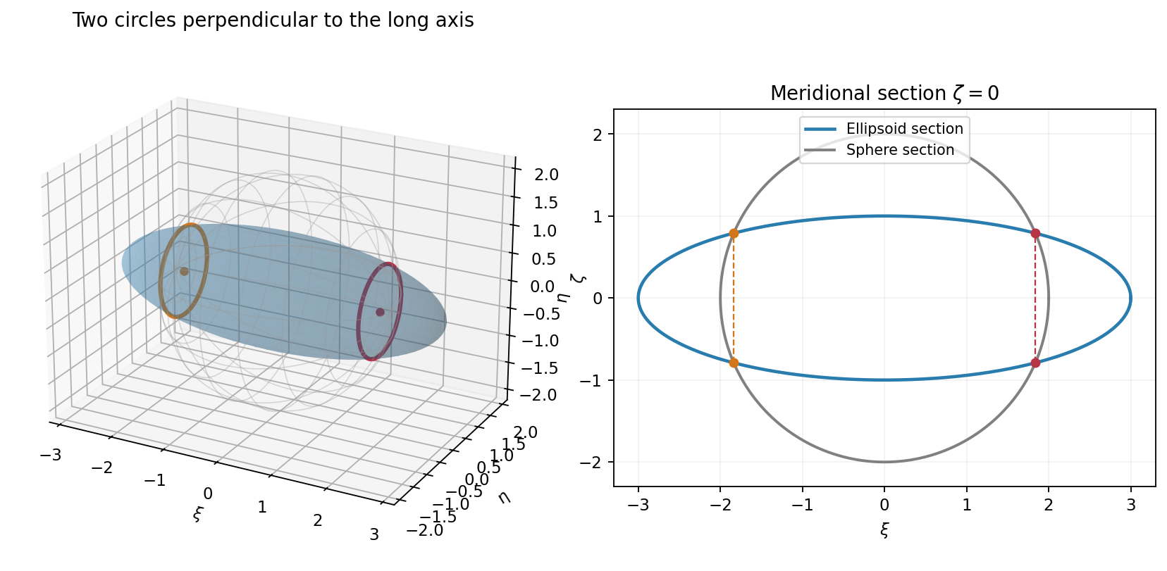
The quadratic-form matrix has eigenvectorswith eigenvalues . In the principal axes coordinates , and , the equation becomesIt is a prolate spheroid, centred at the origin, with semiaxis three along and one in every perpendicular direction. The displayed are one choice of short principal axes.
The sphere has equation . Combining it with the ellipsoid equation givesThe intersection of a prolate spheroid and a concentric sphere therefore consists of two circles in planes perpendicular to . Each has radius , and their centres areTheir plane equations in the original coordinates are .
Minimize or maximize subject to . A Lagrange multiplier givesThe constraint excludes and implies , so it is a regular constraint surface. Multiplying the stationarity equation by gives . Thus the distance extrema on a real quadratic surface satisfyEvery constrained extremum lies in a positive-eigenvalue eigenspace, with squared distance . If is positive definite, the global minimum is and the global maximum is . For an indefinite or singular form the surface need not be bounded; eigenvector directions give stationary candidates, which may be saddles and need not supply both global extrema. With a repeated positive eigenvalue, there can be an entire family of equally distant stationary points.
Complex differentiability requires the same limit for increments along the real and imaginary directions. Real increments give . Imaginary increments giveEquating real and imaginary parts yields the Cauchy-Riemann equationsThey hold throughout the open region where is holomorphic. Conversely, continuous first real partial derivatives satisfying these equations on an open set ensure holomorphy there.
For the real part specified in the PDF,Integrating givesSubstitution into shows . ThusIndeed , so the real part of is exactly the prescribed expression. The arbitrary imaginary constant is the only freedom on a connected domain.
Write and assume its domain is open and connected. If the constant modulus is zero then . Otherwise let . Differentiating this identity and using the Cauchy-Riemann equations givesThese are a linear system for with coefficient matrix , whose determinant is . Therefore , and the Cauchy-Riemann equations also give . It follows thatThis proves the constant-modulus holomorphic function result directly. On a disconnected domain the same conclusion holds separately on each connected component, but the constants can differ.
Partial fraction decomposition give . Let . Each fraction has a geometric expansion, soEquivalently, its coefficient is . The first terms areThe linear and fifth-order coefficients vanish. Both geometric series converge for , and has genuine simple poles at , each distance from the centre. Thus the Taylor series has
At each of , has a simple pole and at most a simple pole. The products and are analytic, so both are regular singular points. More precisely their limiting values are and zero, giving indicial equation , with exponents .
To classify infinity, set and . The transformed equation isAfter division, its coefficients satisfyBoth are analytic at , while itself has a pole. Hence , with indicial exponents . These classifications remain valid at , when the exponents at infinity coincide.
Because zero is an ordinary point, substitute . Matching powers givesEven and odd coefficients evolve independently. Taking and constructs solutionsTheir initial values and derivatives give , so they are linearly independent. These power series of the Chebyshev differential equation span the local solution space. A useful check is and , with at .
For a nonterminating parity series, consecutive nonzero terms satisfyThe ratio test therefore gives for each nonterminating series. The nearest singular coefficient points are , both distance one from the expansion centre.
The polynomial exception is essential here. If is an integer, the series of the same parity as terminates and has ; the opposite-parity independent series remains nonterminating with radius one. For noninteger , both have radius one. A regular singular point can be removable for one particular solution, so its presence does not force every individual solution to have finite convergence radius.
If is an integer, the recurrence has zero numerator at . Choosing the parity containing therefore makes all later coefficients vanish. Conversely, for a nonzero polynomial of degree , the coefficient of in the differential equation is , so is necessary.
Normalizing the terminating series by gives the first Chebyshev polynomials:Substitution verifies each differential equation and endpoint value. More generally, ; its recurrence also establishes polynomiality and the normalization.
For fixed endpoint values and smooth admissible variations, the Euler-Lagrange equation isThe first variation follows by integrating by parts and using at the endpoints.
For the claimed first integral, differentiate directly:Along an extremal the bracket vanishes. Thus when , the Beltrami identity isFor a further regular constraint , introduce a constant Lagrange multiplier and make stationary. Apply the Euler-Lagrange equation to the combined integrand, then impose the endpoints and to determine the integration constants and multiplier.
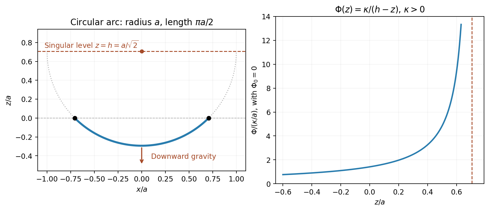
A curve element has arc length and mass . Adding its gravitational energies givesFor the fixed-length constraint, use the augmented integrand . It has no explicit dependence, so the Beltrami identity givesThe desired lower circular arc isIt joins the required endpoints, subtends angle , and has length . Its slope gives . Therefore a gravitational potential producing a circular hanging chain isChoosing makes the first integral constant, . Its gravitational acceleration is , which points downward. An arbitrary additive potential constant changes no force.
This construction really gives a minimum. With , the variable part of is ; the term is fixed by the length. The calibration for semicircular hyperbolic geodesics uses , whose gradient has norm . The Cauchy-Schwarz inequality gives , with equality on traversed left to right. Thus the circular arc minimizes the energy among competitors of the same length and endpoints in the stated potential domain, rather than merely satisfying a necessary stationarity condition.


Let , where for a nonzero admissible real function. Writing , its first variation isChoose boundary conditions making the boundary term vanish, for example homogeneous Dirichlet boundary conditions, homogeneous Neumann boundary conditions, or a corresponding mixed pair. Arbitrary interior variations then give the Sturm-Liouville problemMultiplying this equation by and integrating by parts, with , yieldsThus eigenfunctions are stationary directions of the quotient. The lowest eigenvalue is its global minimum; higher eigenfunctions need not be unrestricted maxima or minima. General Robin boundary conditions require including their boundary energy in the quotient unless the displayed endpoint products also vanish.
The Rayleigh-Ritz method chooses admissible trial functions depending on finitely many coefficients and minimizes this quotient over them. Expansion in a complete orthonormal basis with weight shows , so the trial minimum is an upper bound on the true lowest eigenvalue. In a finite basis, the minimization becomes a generalized eigenvalue problem for the stiffness and weighted mass matrices. Enlarging the trial space can only lower or preserve this upper bound.
For a spherically symmetric function, the Laplacian in spherical coordinates reduces toMultiplying the Helmholtz equation by givesThe endpoint at is singular in Sturm-Liouville terminology; bounded regular radial fields select the physical solution and eliminate the branch. At the field has the imposed zero Dirichlet value. For regular solutions and admissible trial functions, the endpoint term vanishes at the origin and at the wall.
The radial Rayleigh quotient isFor the given trial profile, the numerator is . The denominator isThereforeThe profile is regular at the origin and vanishes at the wall, so it belongs to the admissible trial space. This is the variational estimate for the radial Dirichlet modes of a spherical cavity.
Set for . Direct differentiation gives , so the radial equation reduces toBoundedness of requires , and the wall condition requires . The nontrivial solutions are consequentlyTheir origin values are the removable limits . At , the only bounded radial solution is constant and the wall forces it to vanish, so there is no zero mode. The lowest eigenvalue isIt is below , as required by the Rayleigh-Ritz variational principle. The trial value overestimates by approximately .
Articles by others on the same topic
There are currently no matching articles.