Right multiplication gives a right action . To obtain a homomorphism into permutations with the usual function-composition convention, use the associated left actionThis is well-defined: replacing by , , does not change the image coset. Moreover , and each map is bijective with inverse .
An element is in the kernel precisely when for every . This says , equivalently . HenceThis is the largest normal subgroup of contained in .
Now the index of is , so embeds into . Its order therefore divides . Since is prime, does not divide . From it follows that divides . But and , forcing . Therefore is normal.
For the last case let . Normality makes conjugation by an automorphism, so with . Applying it twice and using gives , so . Thus , andBoth possibilities are allowed; the order assumptions alone do not force the inverse case.
An irreducible polynomial has positive degree, so its ideal is proper: otherwise would contradict degrees. Every nonzero class has a representative not divisible by . Irreducibility gives , and the Euclidean algorithm supplies polynomials with . Passing to the quotient gives . Thus the quotient is a nonzero commutative ring in which every nonzero element has an inverse, hence a field. Constants embed injectively because no nonzero constant lies in the positive-degree ideal .
Polynomial division gives a unique remainder of degree less than in every coset. Thus the classesspan the quotient as an -vector space. A linear combination of them that vanishes would be a polynomial of degree less than divisible by , so it is the zero polynomial. They are therefore linearly independent, proving
Take . Every quotient class is a polynomial expression in with coefficients from , so . Substitution gives . ThusThis constructs a field containing a root even when no root existed in the original field.
First address the general splitting-field request. A splitting field is an extension in which the polynomial factors into linear factors and which is generated over the base field by its roots. For a degree- polynomial, adjoin a root of an irreducible factor. The quotient construction in the preceding parts gives an extension of degree at most . Remove the resulting linear factor and repeat, now with a polynomial of degree over that extension. Induction and the tower law giveThe resulting field is generated by the roots and is a splitting field. Repeated roots or inseparability can only reduce the required degrees; separability was not used.
For the specified cubic, put and . Its splitting field is . Eisenstein criterion at two gives . This cubic field is real and therefore does not contain the nonreal , whose quadratic polynomial is . Consequently
Let . Its odd powers are exactly the four roots, so is the splitting field. The polynomial is irreducible: after the invertible substitution , it becomes , which satisfies Eisenstein criterion at two. HenceEquivalently the field is , since , and .
FactorThe roots are , so the splitting field is . The real quadratic field does not contain , which adds a further degree two. Therefore
A primitive root modulo is an integer whose residue generates the multiplicative group , equivalently has order .
The Chinese remainder theorem states that, for pairwise coprime positive integers , the system has a unique solution modulo . For a constructive proof put . Bézout's identity gives an integer with . Then has all the required residues. If two solutions exist, their difference is divisible by every ; pairwise coprimality makes it divisible by their product, proving uniqueness modulo .
Here divide , and none is zero modulo . Choose a primitive root and exponents withUse the theorem with moduli to choose such that , , . Define nonzero residuesThe exponents are integers; negative ones are interpreted using inverses in . Taking integer representatives now givesThe theorem aligns the exponent modular congruences, which is why a primitive root converts the three power conditions into a linear modular congruence problem.
The monotone convergence theorem states that if pointwise almost everywhere and the functions are measurable, then , allowing the value infinity.
Interpret the displayed densities as zero outside , so no undefined logarithm is evaluated there. Each is nonnegative and measurable. With ,where the last equality is integration by parts. This is finite, proving Lebesgue integrability.
The nonnegative partial sums satisfy, for ,They vanish outside the interval as well. Monotone convergence therefore givesThe series is finite by comparison with the convergent series , whose convergence follows from the integral test. Since , this finite integral proves absolute Lebesgue integrability as required.
We first prove the differentiation theorem. Fix and take nonzero with . The measurable difference quotientsconverge pointwise to . The mean value theorem and the assumed derivative bound give . In particular is measurable as a limit of quotients along a sequence, and its bound by proves integrability. The dominated convergence theorem, in its parameter-limit form, says that pointwise convergence with a common integrable bound permits convergence of the integrals. Applying it yieldsThe parameter-limit statement follows from the ordinary sequential theorem by applying it to every sequence of nonzero tending to zero.
For the specific function, , which is integrable by the allowed fact. It is differentiable in , withThe last majorant has integral one on , using the substitution . All three hypotheses therefore hold. The indicator of the parameter domain is one at every point under consideration and does not affect this derivative.
The theorem givesIntegration by parts has zero boundary term: the sine vanishes at zero and the Gaussian tends to zero at infinity. Hence .
The same Gaussian majorant and dominated convergence give continuity at zero, where the allowed Gaussian integral gives . The differential equation implies ; continuity at zero fixes that constant. Thus
A subset is compact if every cover of it by open sets of the ambient space has a finite subcover; equivalently use open sets of its subspace topology. A cover of separately covers and . Compactness of each supplies two finite collections, whose union is finite and covers . If is closed in a compact space, add the open complement of to any open cover of . Compactness supplies a finite subcover of the whole space, and discarding the complement leaves a finite cover of .
For the enlarged space, every old open set is open in and has the same trace on . The trace on of a new open set is , which is open in because its complement is closed. Thus the induced topology on is exactly the original one.
Given an open cover of , choose a member containing infinity. It has the form with compact. The remaining cover restricted to has a finite subcover. Together with the chosen infinity-neighborhood, these finitely many sets cover . Hence is compact, with no Hausdorff assumption needed.
Finally put . Continuity makes open and containing infinity. Therefore with compact and closed in . For every we haveThis expresses convergence to the value at infinity outside compact closed subsets.
A quotient map is a surjection such that is open if and only if is open in . Thus the topology on is exactly the final topology induced by .
For an open continuous surjection, continuity gives one implication. For the other, if is open then is open by openness and surjectivity. Hence it is a quotient map.
If and are quotient maps, they are surjective andThis set is open exactly when is open, exactly when is open. Thus the composition is a quotient map.
For the factorization, continuity of implies continuity of . Conversely, if is continuous and is open in , then is open. The quotient property makes open. This holds for every open , so is continuous.
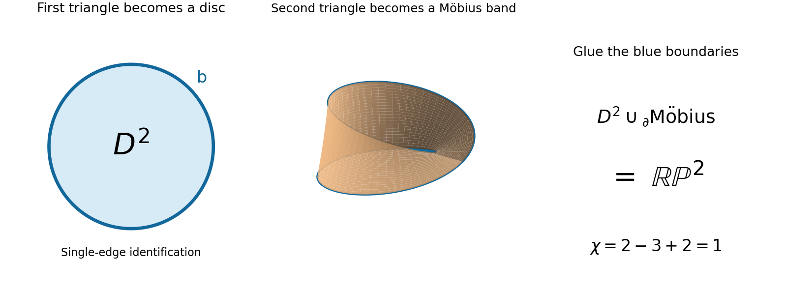
The two singly marked sides of the first triangle are glued with their endpoints at matched. A cross-section parallel to the remaining side has its two endpoints identified, becoming a circle; the apex becomes its cone point. Thus this quotient triangle is a disc, whose boundary is the doubly marked edge.
In the second triangle, the two triply marked sides run consecutively along the boundary from through to . Pairing these sides in the indicated directions introduces one reversal; its boundary word is , where is the remaining doubly marked edge. This is a Möbius band with boundary . One can obtain the usual rectangle model by cutting from the identified triple-edge seam to the midpoint of and opening the triangle.
The double markings glue the disc boundary to the boundary of that Möbius band. Capping a Möbius band by a disc givesThis description also verifies that the quotient is a closed surface, including the vertices. As a check, the vertex classes are and ; there are three edge classes and two faces. The Euler characteristic is , consistent with the projective plane. The Möbius band exhibits nonorientability directly.
The Fréchet derivative at is the linear map satisfyingIt is unique. When both derivatives exist, the chain rule is .
For the square map,The remainder has norm at most in a submultiplicative matrix norm, hence is . ThereforeMatrix multiplication is not commutative, so the two terms cannot generally be combined as .
For small , the matrix remains invertible and its inverse is locally bounded, for example by the convergent Neumann series when . Applying the resolvent identity twice givesThe last term is by that local bound. Hence the inverse map is differentiable, withThis verifies the differentiability and its remainder, rather than only formally differentiating the identity .
First simplify the composite: . Applying the product rule to four factors of , and the preceding inverse derivative to one factor at a time, givesThe four terms have left and right exponents . The same expression follows by composing , and in that order. Only when commutes with can it be simplified to .
Write . At a regular constrained extremal, the first variation of is not identically zero. Choose a variation for which ; the implicit function theorem supplies a correction in the direction to each other variation so that remains one. Stationarity of on these corrected variations implies for one scalar .
Put . Integration by parts gives, for an arbitrary twice continuously differentiable variation ,Taking variations with zero endpoint values and using the stated fundamental lemma of the calculus of variations gives the Euler-Lagrange equation. The remaining endpoint values are free and independent, giving the natural boundary conditions:If the constraint is not regular, the general multiplier statement permits an abnormal pair with ; the source's general normal-form derivation implicitly excludes that case. In its quadratic example, regularity follows automatically from normalization: .
For that example , so the equation and endpoint conditions reduce toMultiply the equation by and integrate. The boundary term vanishes, givingThe last integral equals one, so , the functional value at the constrained extremal.
Finally multiply the equation for by and the equation for by , then subtract and integrate. The derivative terms give only the vanishing boundary term , while the terms cancel. Therefore . For distinct multipliers this proves
Use coordinates with the downward vertical as reference. The first rod's center is at , so its translational plus rotational kinetic energy is . The second center isIts squared speed is . Adding its center-of-mass rotation, using moment of inertia , gives the totalThe two center heights give . Hence is exactly the stated Lagrangian.
Small stable oscillations are about the downward equilibrium . Retaining quadratic terms gives and , whereA normal mode satisfies . With , the determinant equation isThus the angular frequencies areBoth squared frequencies are positive. The amplitude ratio is : it is positive in the lower-frequency mode and negative in the higher-frequency mode. The rods therefore swing in phase in the first mode and in opposite phase in the second.
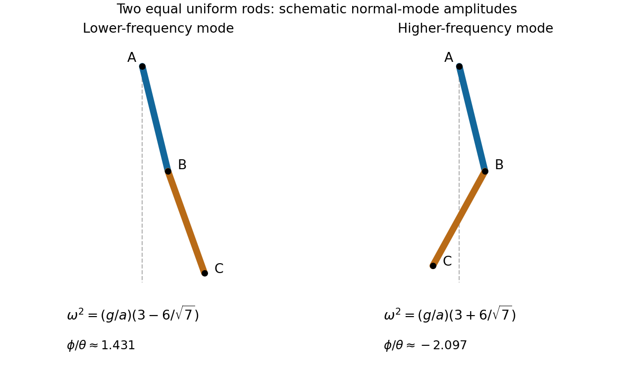
The two-rod normal modes have positive and negative relative angular amplitudes
. Details. In SI units the Maxwell's equations in vacuum, with sources, areTaking the divergence of the last equation and using Gauss's law gives , the local conservation of electric charge. Thus sources that violate charge conservation cannot satisfy all the Maxwell's equations. Equivalently, with this conservation law the curl evolution preserves the electric divergence constraint if it holds initially; Faraday's law similarly preserves .
With , use and substitute the two curl equations. This gives . Applying the same calculation to yieldsA monochromatic plane wave has one angular frequency and constant-phase planes , normal to the wavevector . Its wavelength is .
For a nontrivial traveling wave with , substitution of the displayed electric field into the divergence equation gives . Faraday's law is satisfied byIndeed and . The magnetic divergence is zero, while Ampère's law reduces to , giving the dispersion relation. The amplitudes may be arbitrary transverse vectors; they need not be mutually orthogonal or have equal lengths. Their combination describes the polarization.
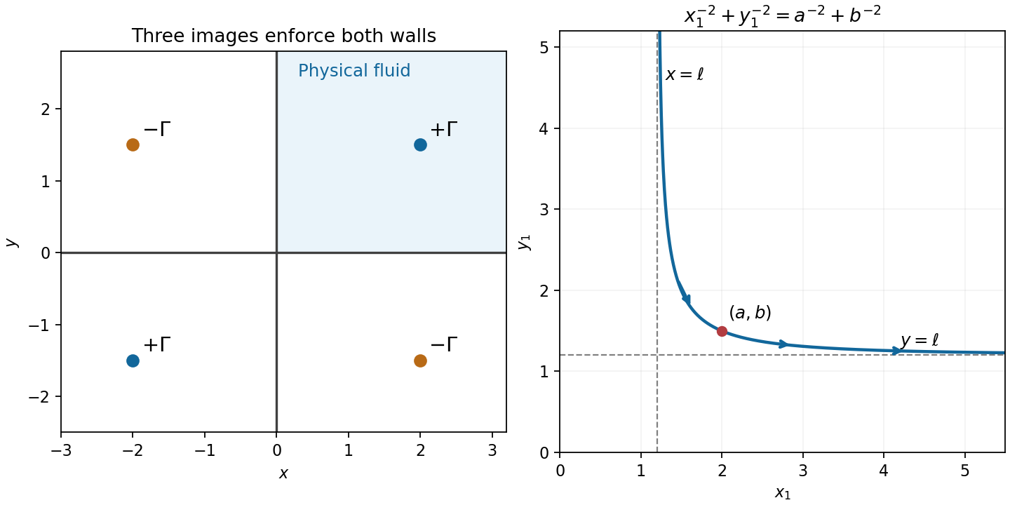
Use the convention that a positive vortex has counterclockwise circulation, with complex potential of a two-dimensional potential flow . To make both coordinate axes streamlines, place images of strength at and , and strength at . The resulting potential isAdditive constants and consistent logarithm branches do not affect velocity. The quotient has unit modulus on either wall, so the streamfunction is constant there and there is no normal flow.
The vortex moves with the regular fluid velocity after removing its own singular field. Since , evaluating the three image contributions at gives exactlyThe overall minus sign and the two reflected-term minus signs here agree with the source scan.
Write , with . Taking real and imaginary parts yieldsDividing gives , which integrates toPut . The first-quadrant branch has vertical and horizontal asymptotes and . Its motion is to the right and downward: from large near the vertical asymptote toward large near the horizontal one. Both coordinates stay strictly positive, so no wall is crossed.


The exact free-surface kinematic condition is evaluated at . Linearizing about a flat surface at rest drops products of small quantities and evaluates at , giving . Bernoulli's equation with constant atmospheric pressure gives to the same order. The rigid bed has no normal flow, hence at .
In the fluid, incompressibility and the velocity-potential representation give . For , takeIt is harmonic, satisfies the bed condition and the linear dynamic condition. At the surface its vertical derivative is , while . Therefore the kinematic condition is equivalent toFinally . Taking the square root givesThe first term is nondispersive shallow-water speed; the next term is the leading finite-depth dispersion correction.
For a joint probability density function, independence is equivalent to almost everywhere. The displayed density is valid for . Complete the square:Integrating the second normal factor over givesDividing the joint probability density function by this marginal yields the conditional lawFor the joint probability density function factors and the variables are independent. If , the conditional mean depends on , so independence fails; equivalently their covariance is .
Define . In the change of variables , the Jacobian cancels the remaining density factor, leaving the product of two standard normal densities. Thus is standard normal and independent of . One choice isChanging both signs gives the other standardized choice. The density transformation proves independence directly rather than inferring it from zero covariance without a joint-normal justification.
The state space is . Write . The nonzero transition probabilities areThe stationary equations give and for . Normalization gives , soThe remaining equation is satisfied, confirming stationarity.
The chain is irreducible: every positive state can jump to zero, and zero can reach every state through consecutive immigration steps. A stationary probability distribution makes it positive recurrent. Returns to zero can have lengths two and three with positive probability, so it is also aperiodic. The Markov-chain ergodic theorem now gives the almost-sure long-run time proportion for as the stationary tail:This time-average conclusion applies to the specified start at zero.
Independent increments give independent Poisson variables and with means and . Dividing their joint probability by yieldsThus the conditional distribution is binomial distribution with parameters .
The event means that at most events have occurred by . ConsequentlyFor , the conditional event time lies in . Integrate its survival function and substitute :The index range is implicit in the source's last assertion. For , the th event is after , and independent future increments instead give expectation ; the displayed formula does not apply.
Minimize . Differentiation gives the normal equations . Full column rank makes positive definite, soThe expectation uses the zero error mean; the covariance uses . With independent Gaussian errors of common variance, maximizing likelihood minimizes exactly the same residual sum of squares, so this is also the maximum likelihood estimator, whether the common variance is known or estimated.
For the quadratic design, decompose each group's residual sum of squares into its within-group constant plus the group size times the squared residual of its sample mean. The three parameter combinations , and can fit all three group means exactly. ThereforeThe group means are independent normal variables, with variances . Hence their two stated linear combinations are jointly normal, andJoint normality therefore proves the two estimators are independent. Their variances are and , respectively. Equal replication at the two off-center temperatures is what cancels the covariance.
A possibly randomized statistical test has rejection probability after observing . Its statistical power at parameter is , and its test size is the supremum of that statistical power over the null parameter set.
For simple hypotheses with densities , the Neyman-Pearson lemma states that a level- test is most powerful if it rejects where , accepts where , and randomizes on equality to obtain null rejection probability . Here is chosen to reach that test size. To prove optimality, let be this test and any test of level at most . Pointwise,Integrating and using gives . This proves maximal statistical power. For , equality also forces any equally powerful test to use all its allowed test size and agree with the indicated decisions away from the likelihood-ratio tie set, up to null sets.
For the Poisson sample, and, for every fixed , the likelihood ratio isIt increases strictly with . Choose an integer so that , and reject for , with boundary rejection probabilityThis has exact test size . Its rejection ordering and calibration do not depend on which is selected, so the lemma proves it uniformly most powerful for the whole one-sided alternative. Randomization is generally needed for an exact arbitrary test size in a discrete model.
For the approximate design, the central limit theorem under gives critical sum . Under , the sum is approximately normal with mean and variance . Target statistical power therefore givesor . Thus the requested design expression isRound upward to obtain an integer design. This is a normal approximation to the requested statistical power, rather than an exact discrete sample-size guarantee; the exact Poisson test above provides its exact calibration.
Define to be identity outside rows and columns , with blockThe block's transpose times itself is identity because and the off-diagonal terms cancel. Thus is orthogonal, with determinant one.
For , choose , . Then , and every other coordinate is unchanged. If , choose . This fixes the useful nonnegative pivot convention.
Apply the rotations to the current matrix in the displayed order from right to left. First eliminates entry ; then eliminates without changing row two. Finally eliminates while preserving the zeros in column one. ThusInverting the product gives . Even if starts lower triangular, the row rotations generally create nonzero entries above the diagonal; there is no further universal simplification. For example gives positive-pivotwhose three entries above the diagonal are all nonzero.
If is orthogonal, is both upper triangular and orthogonal. Orthogonality of its columns successively forces all off-diagonal entries to vanish and all diagonal entries to have absolute value one. The first two pivots are positive under our convention, and the rotations have determinant one. Therefore the precise result isWithout a specified pivot-sign convention, the invariant statement is a diagonal matrix with entries and product .
A cubic spline is a twice continuously differentiable function whose restriction to each knot interval is a polynomial of degree at most three. Its second derivative is continuous and piecewise linear. Natural endpoint conditions are .
Linearity of both the piecewise-polynomial and smoothness conditions, and of the endpoint equations, makes the natural splines a vector space . A continuous piecewise linear second derivative with zero endpoint values is determined freely by its interior nodal values. Integrating twice adds two arbitrary affine constants. HenceThis count includes the case of one interval.
An interpolating spline has at every node. Set , so vanishes at all nodes. On each open knot interval is constant. Two integrations by parts giveThe terms containing vanish at nodes. When summed, the interior terms cancel because and are continuous. The two outer terms vanish by the natural endpoint conditions. ThusIntegrating the given square identity now yields the sharper energy decompositionIn particular the natural interpolating spline minimizes the squared-curvature integral.
If is another natural interpolant, the same minimizing argument in both directions makes the two energies equal. The final nonnegative integral then vanishes, so everywhere by continuity. Their difference is affine and zero at all knots, including the two distinct endpoints, so . This proves uniqueness.
It also supplies existence if needed: nodal evaluation is a linear map from the -dimensional space to . Its kernel is zero by the same argument with zero data and the zero competitor. It is therefore surjective, so every data vector has a natural spline interpolant.
Articles by others on the same topic
There are currently no matching articles.