Source paper: www.whatdotheyknow.com/request/physics_preliminary_examinations/response/1162943/attach/3/Twain.7z?cookie_passthrough=1
This is the ordinary sitting of 8 June 2015. The rubric requires Section A, Questions 1–7, and three of Section B, Questions 8–11; all eleven questions are solved below. The source's capital A–C cases, Roman-numbered parts and nested lettered subparts are preserved.
Take the launch point as and ignore air drag. In projectile motion with constant gravitational acceleration , a launch at angle above the horizontal givesAt the wall , the height isThis is a concave quadratic polynomial in , so its unique maximum satisfies . HenceFor , the best trajectory has and reaches the wall at launch height. For , the mathematical maximum height is negative. If the ball must stay above level ground, it lands before reaching the wall: is the maximum same-level projectile range. If there is no intervening ground and the wall extends below the launch height, the same optimum still applies, but its impact point is below that height.
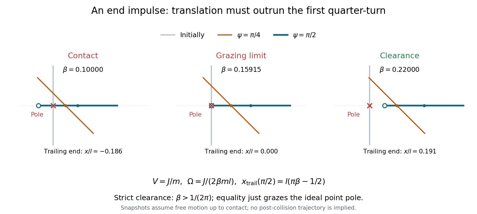
Idealize the pole and stick as having negligible transverse thickness. Put the pole at the origin, the stick initially along the axis, and the struck lower end at , as in the source diagram. A short horizontal impulse along gives the centre of mass a constant speed . The angular impulse about the centre is , giving constant counterclockwise angular velocityThe pole exerts no further force while the stick moves clear of it. Let . The trailing upper end has coordinatesThe pole can lie on the translating straight stick again only when the stick becomes horizontal: for other orientations, its intersection with is the moving midpoint . At the first horizontal orientation, , the trailing end is atConsequently the grazing clearance of an impulsively struck rod occurs atFor the whole stick has passed the pole by its first horizontal orientation, and the continually advancing centre makes all later passes safe. Equality is the limiting grazing contact of the endpoint; strict avoidance requires the strict inequality. If , the pole lies within the stick at that first horizontal pass, so contact occurs before the freely moving trailing end can pass the pole. A uniform thin stick has , below the threshold: sufficient mass near the ends is needed to increase its moment of inertia and reduce the rotation relative to translation.

Take as the constant mass of the sled and rider when snow is immediately removed. Assume the falling snow has zero horizontal velocity in the ice frame, and its arrival rate is the specified constant mass flux onto the sled. In a snow-collecting sled, horizontal momentum flux, including the departing snow, determines the change in sled momentum.
Snow leaves perpendicular to the motion in the rider's frame, so its outgoing horizontal velocity in the ice frame is . During , incoming snow brings zero horizontal momentum and outgoing snow carries . ThusAlthough the sled does not retain snow, it must continually supply the snow's departing horizontal momentum.
Snow now leaves with zero horizontal velocity in the ice frame, the same as its incoming horizontal velocity. The net horizontal momentum flux is zero:Any forward momentum given to the snow on capture is returned to the sled while sweeping it off. “Perpendicular” specifies a different outgoing velocity here than in case A; changing the reference frame without transforming that velocity would miss this difference.
The snow remains aboard, so the moving mass grows as . Incoming snow contributes no horizontal momentum, and there is no horizontal external force. ThereforeThe combined sled–snow system follows a variable-mass system balance; setting would omit the incoming mass term.
Use a circular Earth orbit of radius about the Sun, neglect Earth's rotation, the other planets and atmospheric drag, and treat the launch as an initial impulse followed by unpowered flight of constant mass. DefineIn the patched conic approximation, a surface launch at speed leaves Earth's gravitational field with Earth-relative hyperbolic excess speed , whereThus the necessary solar-orbit change must be supplied in addition to escaping Earth's gravity; simply adding the two escape speeds is incorrect. The asymptotic departure direction can be chosen to minimize . Representative values are and .[ref]
Earth Fact Sheet by National Aeronautics and Space Administration. Orbital parameters: mean orbital velocity 29.78 km/s; bulk parameters: escape velocity 11.186 km/s
To escape the Solar system in the single-Sun approximation, the heliocentric specific orbital energy must reach zero. At Earth's orbital radius, the required heliocentric escape speed is . The smallest change from Earth's initial velocity is prograde, parallel to its motion:Combining the terrestrial and solar energy requirements givesThe asymptotic heliocentric trajectory is a parabolic Kepler orbit; larger launch speeds can give positive solar orbital energy.
Direct fall towards a point Sun. If the Sun is treated as a point target, the projectile must lose its heliocentric angular momentum. The cheapest change is retrograde, cancelling Earth's tangential orbital velocity. It then starts its radial fall with zero heliocentric speed, so andThis is the usual radial-fall estimate. Merely launching towards the Sun while retaining Earth's tangential velocity does not remove the angular momentum barrier.
Minimum for impact on a finite Sun. A literal collision with the solar surface does not require zero angular momentum. The limiting solar impact by a retrograde launch instead has apocentre at Earth's orbit and pericentre at the solar surface. The vis-viva equation with semi-major axis gives the heliocentric departure speedIt remains prograde about the Sun, but the Earth-relative departure is retrograde with . Therefore the surface launch speed for grazing the finite solar surface isHere and .[ref]
Earth Fact Sheet by National Aeronautics and Space Administration. Orbital parameters: semimajor axis 149.598 million km
[ref]Sun Fact Sheet by National Aeronautics and Space Administration. Bulk parameters: volumetric mean radius 695700 km
Slightly reducing the departure speed below makes the trajectory enter the solar surface rather than just graze it. The and values correspond to the explicitly different point-target and finite-radius idealizations, not to two ways of adding escape speeds. These are direct-flight estimates; planetary gravity assists and Earth's rotation are outside the model.Let the projectile's initial laboratory velocity be . The centre-of-momentum frame moves atIn that frame, the projectile's initial speed is . An elastic collision preserves that speed, but can change its direction. Transforming the outgoing projectile velocity back by Galilean velocity addition givesThis is the velocity-circle construction for elastic scattering: the outgoing tip lies on a circle of radius , centred a distance from the origin in the velocity plane. Since , and the origin lies outside this circle. The largest scattering angle occurs when the ray from the origin is tangent to it. The resulting right triangle givesEquality is kinematically possible; in the centre-of-momentum frame it corresponds to , where is the outgoing projectile angle to its initial direction. In particular, a heavier projectile cannot reverse its laboratory direction in an isolated elastic collision with an initially stationary lighter target.
Align both frames' axes with the motion and make their origins coincide at . With moving along at speed relative to , the Lorentz transformation and its inverse arewhere ; the transverse coordinates are unchanged. Along the object's path, . Taking differentials of the inverse transformation givesThis is relativistic velocity addition. For it reduces to the Galilean sum; if , the result is still . Two subluminal positive speeds give a subluminal result.
Work in the parent's rest frame, with . Four-momentum conservation givesso both daughter momenta have magnitude . Their relativistic energy-momentum relations give and . Subtracting these two relations and using the total energy yieldsSubstitution back gives the relativistic two-body decay momentum:The unit vector is not fixed by four-momentum conservation alone. The expression under the square root is the Källén function . The physical two-body decay threshold is ; for massive daughters equality gives zero outgoing momentum. For two massless daughters, each has energy and momentum magnitude .
Let be the equilibrium, so . For , the Taylor expansion of the potential givesAn ordinary small-amplitude simple harmonic motion therefore requires a nondegenerate local minimum, , with the quadratic term dominating the higher terms over the excursion. ThenA local minimum with , such as a quartic minimum, need not give small-amplitude harmonic motion with a nonzero limiting angular frequency. If , the equilibrium is unstable rather than oscillatory.
A central force confines nonradial motion to a plane. In plane polar coordinates, the Lagrangian for isThe azimuth is a cyclic coordinate, so is conserved angular momentum. The Lagrangian has no explicit time dependence, giving conserved energyAt fixed , the radial equation of motion is . The effective potential packages the transverse kinetic energy as a centrifugal term alongside the actual potential energy. It gives a one-dimensional radial problem without introducing an extra physical interaction.
A circular orbit of radius is a stationary point of the effective potential:For , and , this givesThe condition makes the radial force attractive. At , the equation instead requires the fine tuning ; then the centrifugal and potential terms cancel at every radius and there is no isolated restoring minimum. If that equality fails, there is no positive-radius circular orbit for this special power.
Write and keep fixed. The small radial oscillations in a power-law potential have squared angular frequencyThe circular orbital angular frequency has magnitude , so . HenceA restoring radial oscillation exists for , subject to the attractive-force condition in part (b). For the radial stationary point is unstable; is the degenerate boundary. This agrees with circular-orbit stability for a power-law central force, since the actual force is proportional to .
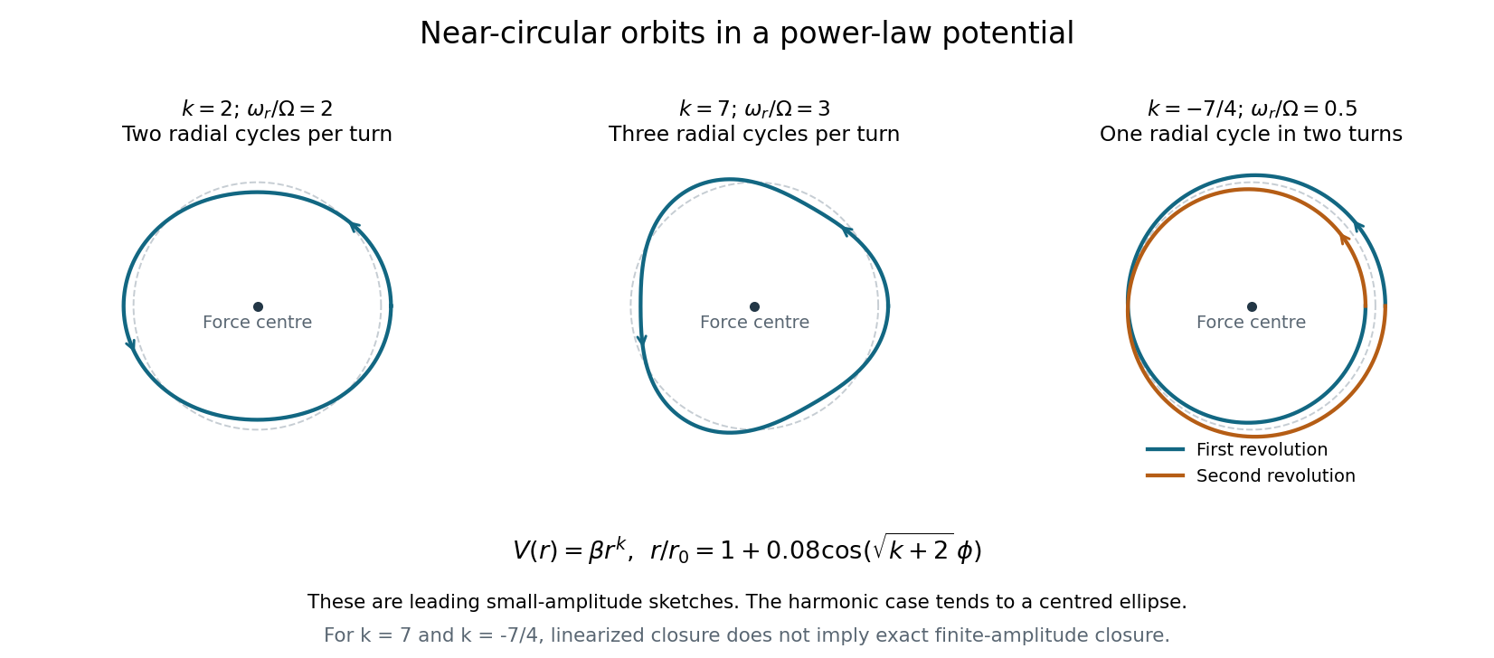
The two positive powers below require ; the negative power requires , so that the force is attractive. To leading order, . The azimuthal advance from one radial maximum to the next isFor , : there are two radial oscillations per revolution. The isotropic harmonic oscillator has orbits that are exact ellipses centred on the force centre, and the perturbed circle is such an ellipse.
For , : the leading perturbation has three radial lobes per revolution, with consecutive radial maxima separated by . Its small-amplitude sketch is a rounded three-lobed orbit.
For , : the radius completes one oscillation while the body makes two revolutions. The leading curve closes after , with a double-wound, generally self-crossing shape; the nearest and furthest points occur in the same spatial direction one revolution apart.
The rational ratios for and describe closure of the linearized near-circular curves. They do not imply that every finite-amplitude orbit closes exactly: higher-order changes in the radial-to-orbital frequency ratio generally produce apsidal precession. Bertrand's theorem identifies the harmonic potential and the Kepler potential as the exceptional attractive central potentials with all nearby bounded orbits closed.

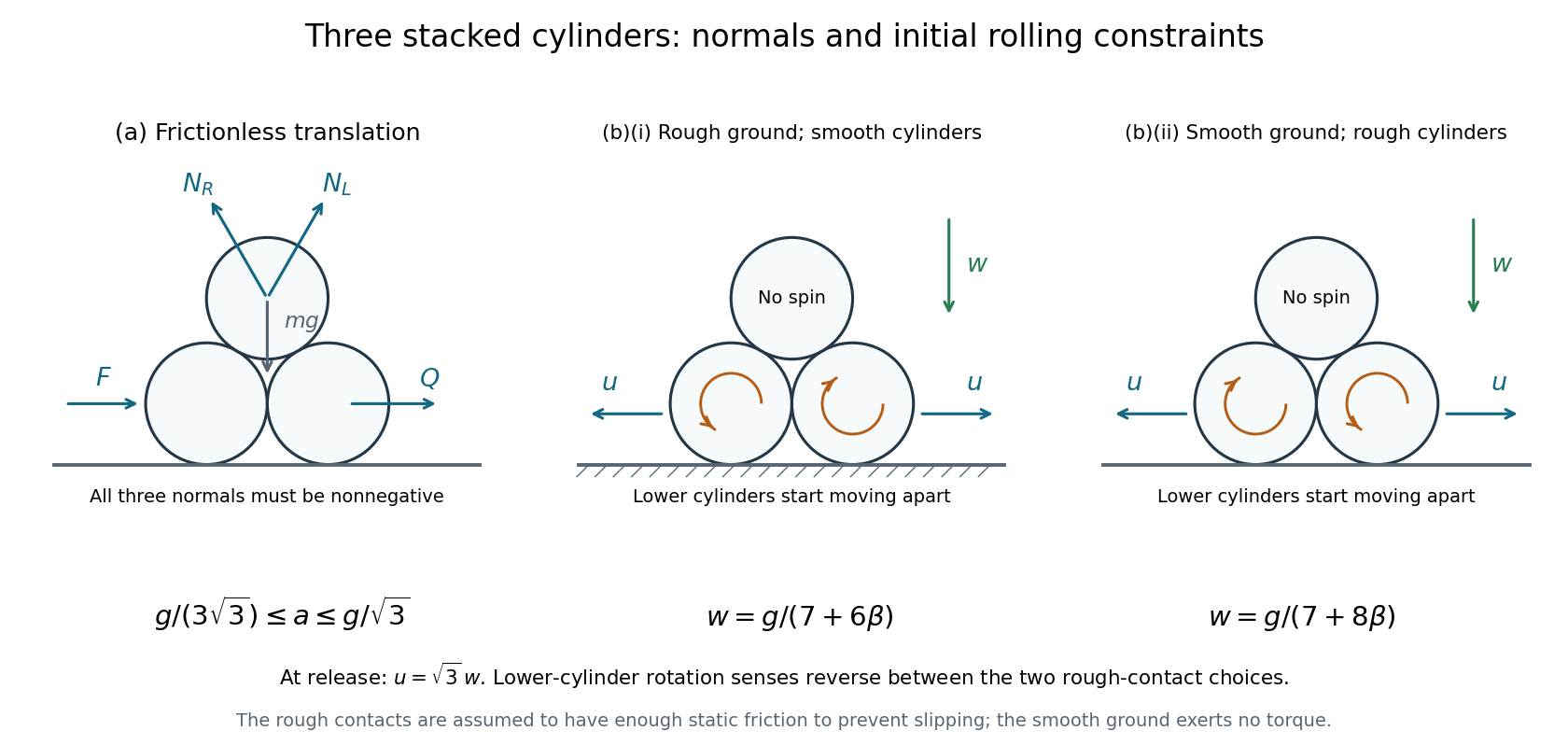
The lines of centres from either lower cylinder to the upper cylinder make with the horizontal. Let be the upward normal forces on the top cylinder from the left and right cylinders, and let be the lower cylinders' mutual normal force. While all three contacts remain closed, the triangular configuration translates horizontally with common acceleration ; frictionless normals exert no torques about the cylinder centres.
For the top cylinder, Newton's second law givesThus and . The right lower cylinder has horizontal equation , soA contact may push but cannot pull: . The limiting inequalities are thereforeAt the lower bound, and the lower pair are just losing compression; at the upper bound, and the upper-right contact is just losing compression. All three pairwise normal forces are strictly positive only inside the open interval. The ground normal forces are positive throughout this range. The applied horizontal force on the left cylinder is , as follows from the whole system's horizontal momentum balance.
Assume the cylinders are released from rest. In each case, “there is friction” is interpreted as sufficient static friction for rolling without slipping at the rough contacts. Without a coefficient or a no-slip assumption, sliding cases would not have a unique specified acceleration. On release the two lower cylinders separate; their mutual contact must not be retained as a rigid constraint.
Let the top cylinder's initial downward acceleration be , and each lower cylinder's outward horizontal acceleration be . The top cylinder initially has no horizontal acceleration. Differentiating the fixed upper-to-lower centre separation twice at the initial zero velocity givesBy reflection symmetry the top cylinder has zero angular acceleration, while the lower cylinders rotate in opposite senses.
Rough ground, smooth cylinder contacts. Let be either upper-to-lower normal force, and the magnitude of the inward ground friction force on each lower cylinder. Pure rolling on the ground requires . The torque equation about a lower cylinder's centre isThe outward translation equation is , giving . The top cylinder's vertical equation is . Using yieldsFor uniform solid cylinders, and . The left lower cylinder rotates counterclockwise while rolling left; the right rotates clockwise while rolling right.
The assumed no-slip ground contact is possible if its coefficient of static friction satisfies at release. This follows from and ground normal force .
Smooth ground, rough cylinder contacts. Write for the tangential contact force magnitude at each upper-to-lower contact. On the top cylinder, its tangential components point upward and outward, while their horizontal components and torques cancel by symmetry. For a lower cylinder, the tangential force has an inward horizontal component and a downward vertical component .
The rolling condition is now at the contact between cylinders, not at the ground. At the initial zero velocity, equality of the tangential contact-point accelerations givesThus gives . The lower cylinder's outward translation equation and the top cylinder's downward equation areUsing gives and henceFor solid cylinders this is . Here the left lower cylinder rotates clockwise while moving left, and the right rotates counterclockwise while moving right. They may slip freely on the smooth ground, so imposing the ground-rolling relation would be incorrect. No slip at the cylinder contacts requires initially.
These are the two cases of the initial acceleration of three stacked cylinders. As a check, as the rotational contribution disappears in both formulas and they approach the smooth-contact release result .

Let the pivot's prescribed horizontal position be and measure from the downward vertical. The bob's coordinates are and . ThereforeWith zero gravitational potential energy at pivot height, the bob's Lagrangian isHere is a prescribed input, not yet a free coordinate. Terms depending only on that prescribed time function can be dropped without changing the equation. The moving block's own kinetic energy becomes relevant when its motion is free in part (d).
The Euler-Lagrange equation for isFor small angles, set and . With and , the harmonic forcing of a horizontally driven pendulum obeysFor , its general solution isThe constants set the initial angle and angular velocity. If the bob starts vertical with zero angular velocity at , this reduces toThe solution remains an approximation only while the resulting angle is small.
As approaches , the driving motion couples resonantly to the pendulum. The particular-solution amplitude has denominator , so a steady harmonic-response formula alone is singular. For a specified finite initial state, the near-resonant motion instead develops beats, and its exact resonant limit has a growing envelope.
For example, with the vertical zero-angular-velocity initial condition above, taking the limit givesThe ideal undamped linear theory predicts amplitude growing linearly with time, not an infinite displacement at the first instant. In reality the motion leaves the small-angle regime, and damping and nonlinear changes of the pendulum's oscillation period alter the response. Below and above resonance, the sign of the harmonic response coefficient changes, corresponding to a phase reversal.
When the block is free, becomes a dynamical generalized coordinate and its kinetic energy must be included. Expanding to quadratic order about the downward stationary state and dropping a constant givesThe coordinate is cyclic. Its conserved canonical momentum is the total horizontal momentum,The two linear Euler-Lagrange equations areEliminating givesThus the pendulum with a freely sliding support has a zero-frequency translational mode and an oscillatory mode. With four independent constants , the general solution isHere and is the horizontal centre of mass coordinate to first order, since . The oscillation is faster than that of a pendulum with a fixed pivot; the limit restores .
Take the natural release interpretation: both block and bob are initially at rest, the block starts at , and the bob has small horizontal displacement relative to the downward line through the pivot. Then , andThe bob's horizontal position isThe block and bob therefore oscillate in opposite phase about the fixed horizontal centre of mass . Their horizontal oscillation amplitudes are and respectively. They pass the centre-of-mass line together when the rod is vertical. If the bob were also given an unspecified initial velocity, the additional sine and translational terms in part (d) would be needed; the source's displacement-release case selects the cosine solution.
Use the tunnel frame , with the entrance at , the far end at , and at both runner entry and photon emission. The runner has , while the approaching photon has . At detection,For , : the photon meets the runner before the runner reaches the tunnel midpoint.
Let be the runner's inertial frame, with origin at the entry event. The Lorentz transformation isThe emission event has coordinates , . It is earlier than entry in : entry and far-end emission are simultaneous only in the tunnel frame. This is relativity of simultaneity, not an extra delay of the light source.
The entrance clock is at . Let be the event on that clock simultaneous with emission in the runner's frame. Since , its reading isThis is the tunnel clock's reading, not the runner-frame coordinate time . It is also not a calculation of what a photograph of that distant clock would show, which would require an additional light-travel condition.
At that simultaneous entrance-clock event, and . Its runner-frame position isThe runner is at , so the entrance is still ahead by distance at the runner-frame emission time. The simultaneously measured distance between the two tunnel ends is , consistent with length contraction.
The photon starts at and travels left to the runner at the fixed position . ThusThis distance is not the simultaneous contracted tunnel length , because the runner is not at the entrance when the photon is emitted in . Adding the entrance-to-runner gap from part (ii) to indeed gives .
During the photon's runner-frame flight, the tunnel entrance moves left by . It began ahead of the runner by , so at detection it lies behind byDivide this distance into the tunnel by the simultaneously measured tunnel length :The runner is stationary in , but their location relative to the moving tunnel still has this fraction. Omitting the initial entrance gap would incorrectly count the runner's progress from an emission event at which they had not yet entered in this frame. These simultaneous positions give the tunnel photon timing in two inertial frames.
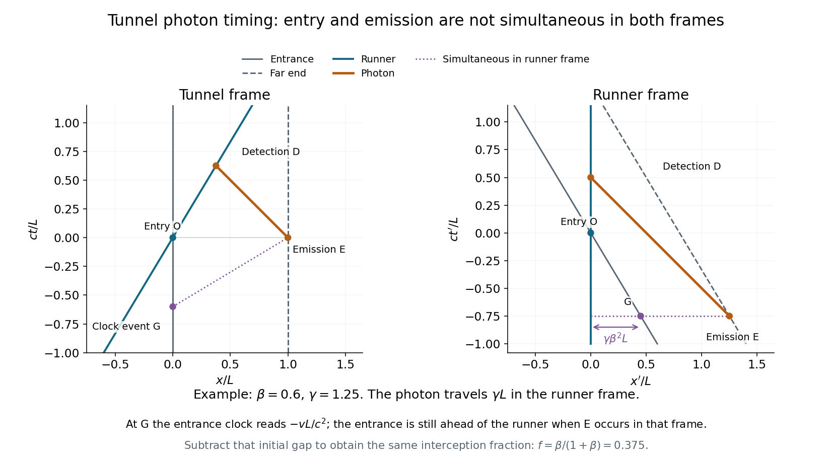
Emission, entry and detection in the tunnel and runner frames
. Original spacetime diagrams for , in units . Event G is on the entrance clock and simultaneous with far-end emission in the runner frame. The runner-frame diagram shows the entrance initially ahead of the runner, and a photon travel distance rather than . Details.
The photon propagates along in the tunnel frame and has energy and momentum . A Lorentz transformation into the approaching runner's frame givesSince , the approaching-source relativistic Doppler effect isIt is a blueshift. With , solving givesThis shift depends on the relative velocity along the light ray, not on the tunnel length or the location of detection.
Articles by others on the same topic
There are currently no matching articles.