Source for this section: Physical PDF pages 271–272, printed pages 7–8 of Physics B (2A), 2 June 2010.
A normal mode has all displacement coordinates proportional to a common time dependence, with fixed relative amplitudes. For a nonzero frequency the time dependence is sinusoidal. A zero-frequency mode is a free displacement or uniform drift rather than an oscillation.
Use the printed mass ordering . Displacements are measured from the unstretched equilibrium positions, givingEquivalently,This is the generalized eigenvalue problem for normal modes of three masses connected by two equal springs. Substitute to obtain . Reflection symmetry gives an antisymmetric vector and symmetric vectors . The former has . For a symmetric vector, the end and centre equations give and . Their solutions are , , or , . HenceThese are all three eigenmodes. The last two keep the centre of mass fixed and are orthogonal in the mass-weighted inner product. The general zero-mode contribution is , accounting for both a centre-of-mass shift and a conserved total momentum. There are no fixed end springs in this system.
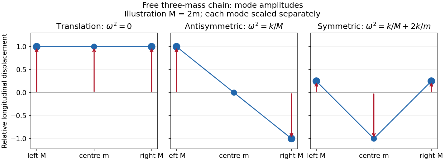
Free-chain mode shapes
. Details. The original amplitude profiles illustrate ; the symmetric internal shape is rescaled for display. The formula above gives every positive mass ratio.
Two further physical examples are standing-wave modes of a string fixed at both ends, with spatial shapes and frequencies , and electrical normal modes of two coupled LC circuits, in which the capacitor charges oscillate at fixed relative amplitudes. Independent normal mode coordinates simplify both systems in the same way as the spring-chain eigenvectors.
A Fourier series separates a periodic physical signal into harmonics. For example, a periodic voltage applied to a linear circuit can be treated one frequency at a time; the harmonic responses then superpose to give the output waveform.
Write for the pulse width and for its duty cycle, with . The waveform is a train of positive rectangular pulses centred on , each with area one. It is even about , so every sine coefficient vanishes. Cosine orthogonality givesand, for ,This is the Fourier series of a periodic rectangular pulse:The actual constant term in the series is , not . As usual for a jump discontinuity, the series converges to the average of the one-sided values at each pulse edge, namely , irrespective of the value assigned at that isolated endpoint. Elsewhere it converges to the rectangular waveform.
Counting the constant as the first term, the first three terms areso their sum isIf “first three” instead means the first three nonconstant harmonics, add ; the original plot shows that alternative partial sum as well. The three-term approximation rounds the narrow peaks and ripples between them; many harmonics are needed to represent a sharp pulse.
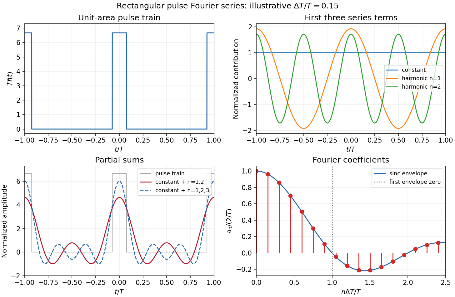
The original sketches use the illustrative duty cycle and cover . The coefficient panel also displays the first spectral zero.
For , expand the sinc function:Thus the low-index coefficients, including , have nearly equal values, although their constant-series contribution still has the factor . The first sinc zero occurs at , or . If this is not an integer, the closest integer coefficient is near zero rather than exactly zero: writing gives . This pulse-width scale of Fourier coefficients means that a narrower pulse requires significant harmonics extending to proportionally larger indices, the reciprocal time-width/frequency-width relation.
Linearity means that the differential operator obeys . Therefore any linear combination of homogeneous solutions is again a solution; associated initial or boundary data must be combined by the same rule.
With characteristic coordinates and , the equation becomes . Integrating in these coordinates givesThe two profiles propagate without changing shape at speeds and . Equivalently write . At , the data imply and . Hence is constant; its two contributions cancel in , givingThe slope formula holds classically wherever the two derivatives exist, and as a weak derivative otherwise. Since the string tension is , here must be mass per unit length. These are two-sided string data with zero slope. The stipulated boundary data specify incoming as well as outgoing waves; this is not a pulse generated on an everywhere initially resting infinite string. For example, at a positive observation point its incoming signal can begin before the motion at begins.
For explicit profiles put , andThen and . At ordinary points, for and zero for . Because itself vanishes at both support edges, this first weak derivative has no delta-function term, although it has jumps.
At , the displacement isFor non-front times its slope isThis is displacement cancellation without slope cancellation in crossing pulses: displacement cancels throughout the overlap , but slope generally does not. Cancellation at one spatial position for an interval of time does not imply cancellation of the spatial derivative there. At , the classical slope is not defined; the adjacent pieces specify its one-sided limits.
At the two windows meet without an open overlap. Their displacements combine intowith slopeAt the classical slope is undefined. At the exceptional meeting time , oddness of gives for every , so the spatial derivative is exactly zero there. Its one-sided time limits at are and ; these do not determine its value at the meeting point.
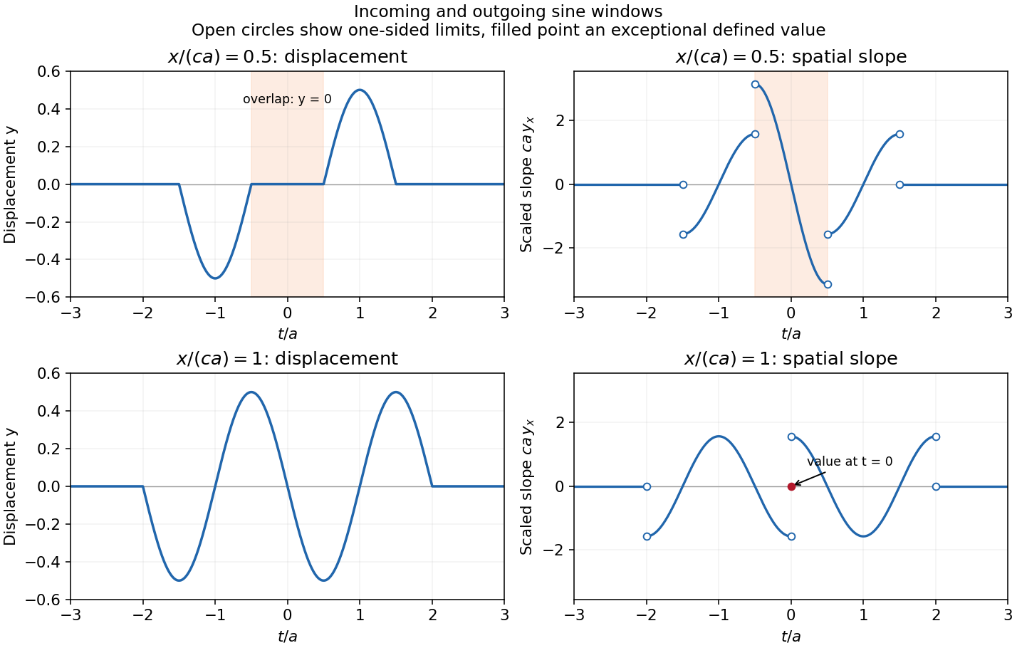


The original graphs distinguish continuous displacements, open-ended one-sided slope traces, and the zero slope at the isolated meeting point. The sharp temporal window is not differentiable at its endpoints, so the overall solution is piecewise classical and globally weak. In particular the literal boundary slope at is not a classical derivative: the even spatial profile has a cusp there. The zero-slope boundary prescription is satisfied at regular times and in its almost-everywhere trace sense; it cannot be read as a globally smooth classical condition for this nonsmooth .
Stokes theorem converts circulation around an oriented boundary into curl flux through a spanning surface. For a sufficiently smooth vector field on an oriented piecewise smooth surface ,The boundary orientation follows the right-hand rule relative to . The field must be smooth on the surface, not merely on its boundary; a singularity crossing the surface cannot be ignored. For a fixed loop, applying the theorem to Faraday's differential law gives the integral flux law of induction.
The planar form is Green theorem. For a region with positively oriented boundary and sufficiently smooth ,The outer boundary is counterclockwise and any holes have clockwise boundaries. For instance makes the area of equal to half the line integral of ; the unit circle gives area .
A closely related use of “Green's theorems” in field theory is Green's identities, obtained by applying the divergence theorem to :and, after subtracting the expression with exchanged,These relate interior sources to boundary data in electrostatics and other boundary-value problems. For example, a harmonic potential difference vanishing on a Dirichlet boundary condition has zero integral of its squared gradient by the first identity, establishing uniqueness. Both the planar circulation theorem and the field identities are included here to make the convention clear.
Separation of variables replaces a compatible partial differential equation by ordinary differential eigenvalue equations. For example, with a thermally diffusive rod, , try . Wherever division is valid,The two sides depend on independent variables, so each must be constant. Homogeneous end temperatures give and . The general initial-temperature profile is represented by superposing these separated modes:Each spatial mode decays at its own rate. For a fixed-end wave equation the same spatial eigenfunctions instead have oscillatory time factors , with coefficients fixed by initial displacement and velocity. Similar constructions separate Laplace's equation in suitable coordinate systems.
A single product is usually only one mode, not the most general solution. Linear superposition and completeness of the spatial eigenfunctions are what extend the method to general allowed data. Nonhomogeneous boundary values can first be removed by a known stationary or particular solution. Separation is effective when the geometry, coefficients and boundary conditions admit a common separated eigenproblem; an arbitrary nonlinear equation or inseparable geometry need not do so. Self-adjoint Sturm-Liouville problems explain the weighted orthogonality and completeness in many physical applications.
Convolution describes the response of a linear time-invariant system to an arbitrary input. If is its impulse response and its input,This is a weighted sum of responses to shifted impulses. For integrable functions the operation is commutative and associative. A causal system has for , restricting the integral to past inputs. With the Fourier convention , the convolution theorem gives .
For example, an RC low-pass frequency response has and , where is the Heaviside step function. Fast input variations are smoothed. The same mathematics describes optical blurring by a point spread function and many other linear response measurements.
Deconvolution tries to recover from measured and known . In noise-free data one formally sets where . Zeros of lose corresponding information; small values amplify measurement noise. If the measured spectrum is , the direct estimate has error , which can be very large at frequencies strongly suppressed by the instrument. An inverse is therefore not automatically unique or stable.
One regularized spectral deconvolution reconstruction isThis minimizes at each frequency and limits noise amplification, at the cost of bias and lost resolution. Choosing the regularization requires assumptions about noise and the desired signal; deconvolution cannot restore components that the data do not determine without such additional information.
Orthogonality means zero inner product, not merely that two objects look different. For complex vectors, ; for functions a common choice is with positive weight . An orthonormal set has .
For an orthogonal set, the component of along has coefficientA complete orthonormal set gives in the appropriate norm and Parseval's identity . Without completeness there can be a nonzero residual orthogonal to the entire chosen set. Orthogonal nonzero vectors are linearly independent, but independence alone does not imply orthogonality.
Fourier coefficients are projections becauseLikewise, for a self-adjoint operator, gives , so distinct eigenvalues have orthogonal eigenvectors. Degeneracy does not itself force a chosen pair to be orthogonal, but an orthonormal basis can be selected within each eigenspace. The differential version uses the correct Sturm-Liouville weight and boundary conditions.
For mechanical normal modes with unequal masses the relevant inner product is . This makes the modes in D14 orthogonal even when an ordinary unweighted dot product does not. Expanding in such coordinates diagonalizes the kinetic and potential quadratic forms, explaining why modal motions evolve independently and their energies add.
Articles by others on the same topic
There are currently no matching articles.