Past exam of the physics B course of the University of Cambridge / 2011 / Paper 1 / Section B

Gauss's law connects electric flux through a closed surface to its enclosed charge:The differential form follows from the divergence theorem. The law is exact; extracting a field magnitude by simple division additionally needs symmetry. For spherical symmetry, $E_r(r)=Q(r)/(4\pi {ϵ}_0{r}^2)$; a uniformly charged ball therefore has a field linear in $r$ inside and an inverse-square field outside. An infinite line of linear charge density $\Lambda$ gives $E_r=\Lambda /(2\pi {ϵ}_{0}r)$ by a cylindrical surface. A uniformly charged infinite sheet gives $E=\sigma /(2{ϵ}_0)$ on either side by a pillbox.

An electrostatic conductor has zero interior field and constant potential; excess charge occupies its surface. A pillbox gives $E_{n,\mathrm{out}}=\sigma /{ϵ}_0$ when the inside is conducting. More generally, $\hat{\mathbf{n}}\cdot ({\mathbf{E}}_2-{\mathbf{E}}_1)=\sigma /{ϵ}_0$. For dielectric matter, $\nabla \cdot \mathbf{D}={\rho }_{\mathrm{free}}$ separates bound polarization charge from free charge. Gauss's law alone does not establish a uniform field for an arbitrary finite plate or recover a detailed nonsymmetric charge distribution from one flux measurement.

An electric dipole has equal and opposite charges separated by a small vector from negative to positive, with electric dipole moment $\mathbf{p}=q\mathbf{d}$. More generally, a localized neutral distribution has $\mathbf{p}=\int {\mathbf{r}}^{\prime }\rho ({\mathbf{r}}^{\prime })d^3{r}^{\prime }$, independent of origin. At distances large compared with its size, the leading nonzero term in the multipole expansion isThe field points along $\mathbf{p}$ on either axial side and opposite $\mathbf{p}$ in the equatorial plane; its axial magnitude is twice the equatorial magnitude at equal radius. Near the charges the finite-charge expression must replace the far-field approximation.

A permanent dipole in an externally imposed slowly varying electrostatic field has interaction energy $-\mathbf{p}\cdot \mathbf{E}$, torque $\mathbf{\tau }=\mathbf{p}\times \mathbf{E}$ and force $\nabla (\mathbf{p}\cdot \mathbf{E})$ for fixed $\mathbf{p}$. A uniform field aligns it but gives no net force. For a linearly induced dipole $\mathbf{p}=\alpha \mathbf{E}$, the formation-inclusive energy is $-\alpha E^2/2$, not $-\alpha E^2$: the moment itself grows while the field is applied. Dipole density gives electric polarization, whose bound charges are ${\rho }_b=-\nabla \cdot \mathbf{P}$ and ${\sigma }_b=\mathbf{P}\cdot \hat{\mathbf{n}}$.

For a fixed circuit, Faraday's law of induction readsSurface orientation and contour direction obey the right-hand rule. The negative sign is Lenz's law: a passive induced current acts against the flux change, consistently with energy conservation. The induced electric field generally has nonzero curl and cannot be represented by one single-valued electrostatic potential.

For a material circuit moving with local velocity $\mathbf{u}$, the measured electromotive force includes the magnetic Lorentz force on its carriers:This distinguishes transformer induction in a stationary coil from motional induction in a changing circuit. A straight sliding rod of length $l$ moving perpendicular to itself and to uniform $B$ has $|\mathcal{E}|=Blv$. With circuit resistance $R$, the electrical power $(Blv{)}^2/R$ equals the external mechanical power needed to oppose magnetic drag. An ideal transformer gives $V_2/V_1=N_2/N_1$ in magnitude from common flux linkage; real leakage, resistance and core losses limit that simple result. pickup coils measure flux change rather than an absolute static magnetic field, so integration and a reference state are needed to recover a field history.

In charge- and current-free vacuum, Maxwell equations reduce toTaking a curl and using $\nabla \times \nabla \times \mathbf{E}=\nabla (\nabla \cdot \mathbf{E})-{\nabla }^2\mathbf{E}$ givesand the same wave equation for $\mathbf{B}$. For a plane wave $\mathbf{E}=\mathrm{Re}[{\mathbf{E}}_0{e}^{i(\mathbf{k}\cdot \mathbf{r}-\omega t)}]$, $\omega =ck$, $\mathbf{k}\cdot {\mathbf{E}}_0=\mathbf{k}\cdot {\mathbf{B}}_0=0$ and ${\mathbf{B}}_0=\hat{\mathbf{k}}\times {\mathbf{E}}_0/c$. Thus the fields are transverse, mutually perpendicular and in phase; polarization describes the electric-field trajectory at a fixed point.

The energy density and Poynting vector areFor a linearly polarized sinusoid with peak electric amplitude $E_0$, the mean intensity is ${ϵ}_{0}c{E}_0^2/2$. Electromagnetic momentum density is $\mathbf{S}/c^2$; normal absorption produces radiation pressure $⟨S⟩/c$, while ideal retroreflection doubles it. Linear superposition permits interference and standing waves, whose local electric and magnetic fields need not have the traveling-plane-wave equality point by point.

The microscopic magnetic response becomes a macroscopic field problem through the magnetization $\mathbf{M}$, the magnetic dipole moment per unit volume. Definein magnetostatics. Bound currents are represented by ${\mathbf{J}}_b=\nabla \times \mathbf{M}$ and surface current ${\mathbf{K}}_b=\mathbf{M}\times \hat{\mathbf{n}}$. Normal $B$ is continuous across an interface, while $\hat{\mathbf{n}}\times ({\mathbf{H}}_2-{\mathbf{H}}_1)={\mathbf{K}}_{\mathrm{free}}$. It is generally incorrect to impose continuity of every component of both fields. A linear isotropic material has $\mathbf{M}=\chi \mathbf{H}$ and ${\mu }_r=1+\chi$, but a ferromagnet usually requires a nonlinear, history-dependent constitutive relation.

Internal field differs from externally applied field. For uniform magnetization along a principal axis of an ellipsoid, the demagnetizing field is $-N_{d}M$ and $H_{\mathrm{int}}=H_{\mathrm{applied}}-N_{d}M$. A linear specimen therefore has apparent susceptibility $\chi /(1+N_d\chi )$ relative to the applied field. Shape is especially important for large susceptibility. A long closed magnetic circuit reduces stray fields; a bar magnet still has demagnetizing fields despite the absence of magnetic monopoles. Equivalent magnetic-pole descriptions are bookkeeping for magnetization divergence, not free magnetic charge.^[ref]

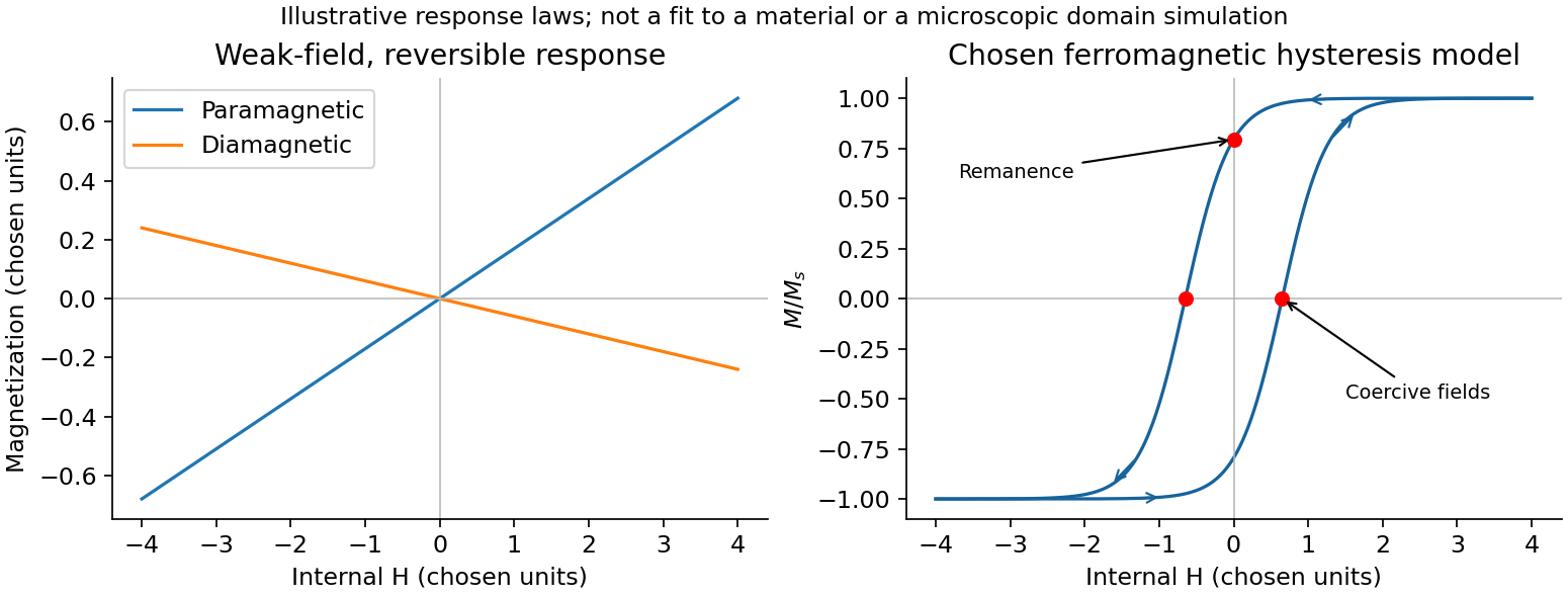
In paramagnetism, permanent localized moments are preferentially aligned by the field, against thermal disorder. For independent spin-one-half moments with projections $\pm \mu$, the two Zeeman energies givein the dilute weak-field limit with $B\simeq {\mu }_{0}H$. This is a Curie law; the response saturates at $n\mu$ when alignment dominates. More generally, spin $J$ gives $\chi ={\mu }_{0}n(g{\mu }_B{)}^{2}J(J+1)/(3k_{B}T)$. Interactions can produce a Curie–Weiss response $C/(T-\Theta )$ over a suitable range. Conduction-electron Pauli paramagnetism need not show the localized-moment $1/T$ law.

In diamagnetism, the field induces a magnetic moment opposing it, so the linear susceptibility is negative. The microscopic cause is the change in orbital electronic motion, and a closed-shell insulating material has no permanent atomic moment to orient. This weak response is often only mildly temperature dependent away from other transitions. It also exists as a background in materials with a stronger positive response. Perfect flux expulsion in a superconductor is a distinct collective phenomenon and should not be identified with ordinary weak atomic diamagnetism.

In ferromagnetism, exchange interactions stabilize spontaneous magnetic order below the Curie temperature. A specimen can have zero net moment while its magnetic domains remain locally magnetized in different directions. Domain-wall motion and moment rotation produce a large response; anisotropy and pinning lead to remanence, coercivity and hysteresis. Increasing field eventually approaches saturation. Heating above the ordering transition removes spontaneous order, although an applied field still induces a response. Soft magnetic cores favor easy reversal and small cyclic loss; hard permanent-magnet materials favor retained magnetization and resistance to reversal. These properties concern collective order and barriers, not merely independent moments all following a weak field.^[ref]

A practical distinction requires a controlled field sweep and a separate magnetic readout. A toroidal core with drive winding $N_1$, path length $l$ and current $I$ has approximately $H=N_{1}I/l$. A pickup winding measures ${\mathcal{E}}_2=-N_{2}AdB/dt$; integrating after calibration gives $B$, and $M=B/{\mu }_0-H$. Reversing the sweep reveals a loop whose positive loss area per volume is $\oint HdB$. An air-core/empty-holder reference, known geometry and turn count, offset correction, temperature control and slower sweeps test background, heating and rate-dependent eddy-current losses. A single force or susceptibility reading cannot establish spontaneous order or hysteresis. The original curves below are illustrative responses, not measured material data.

A galilean transformation relates inertial frames in uniform relative translation. For $\mathbf{V}$ the velocity of the primed origin,Absolute time and invariant acceleration make Newton's second law retain its form for the usual nonrelativistic interactions. For a particle of mass $m$, ${\mathbf{p}}^{\prime }=\mathbf{p}-m\mathbf{V}$ and $K^{\prime }=K-\mathbf{V}\cdot \mathbf{p}+m{V}^2/2$. Momentum and kinetic energy are frame dependent, although an isolated system's conservation laws hold in either inertial frame. Relative velocities and collision predictions are consistent between frames. A rotating or accelerating frame instead requires inertial-force terms. Maxwell equations with a fixed light speed are not Galilean invariant; Lorentz transformations replace these relations when relativistic effects matter.

Kepler's laws of planetary motion state that, in the relative two-body description, bound trajectories are ellipses with the attracting body at a focus, the radius vector sweeps equal areas in equal times, and the square of the period is proportional to the cube of the semimajor axis for a fixed total mass. Their Newtonian derivation is especially informative. With relative coordinate $\mathbf{r}$ and ${\mu }_g=G(M+m)$, the inverse-square acceleration is $-{\mu }_g\mathbf{r}/r^3$. Its zero torque conserves $\mathbf{h}=\mathbf{r}\times \dot{\mathbf{r}}$, fixing a plane and the areal velocity $h/2$.

For $u=1/r$, the orbit equation is $u^{\prime \prime }+u={\mu }_g/h^2$ as a function of polar angle. ThereforeBound negative-energy motion has $0\le e<1$ and semilatus rectum $h^2/{\mu }_g=a(1-e^2)$. Dividing ellipse area by areal velocity givesFor a planet much lighter than its star, replace $M+m$ by $M$. Zero-energy and positive-energy encounters are parabolic and hyperbolic rather than periodic ellipses. Perturbations from other bodies and departures from point-mass Newtonian gravity can precess or otherwise modify the orbit; Kepler's laws are a two-body approximation, not an exact rule for every observed planetary path.

A tidal force measures the difference of gravitational acceleration across an extended object. A freely falling reference frame removes a spatially uniform acceleration, but not its gradient. For a distant point mass $M$ at distance $R$ and direction $\hat{\mathbf{n}}$ from the reference centre, a small internal displacement $\mathbf{x}$ givesThe tidal tensor has eigenvalues $2GM/R^3$ radially and $-GM/R^3$ in each transverse direction: radial stretching and transverse squeezing. Its trace vanishes in the source-free region, consistent with the gravitational Gauss law. An associated relative potential is ${\Phi }_{\mathrm{tide}}=-GM[3(\hat{\mathbf{n}}\cdot \mathbf{x}{)}^2-x^2]/(2R^3)$.

The scale is $GMl/R^3$ across size $l$, not the centre's absolute gravity $GM/R^2$. This distinction explains how a more distant massive object can exert a large force but a modest tide. Opposite-side stretching supports the elementary two-bulge picture; real ocean tides also involve rotation, basin geometry and fluid dynamics, so the static gradient alone does not predict coastal heights or timing. The same gradient stresses satellites and can disrupt a self-gravitating body when it competes with the body's own gravitational restoring acceleration.

A rapidly spinning gyroscope approximately has angular momentum $\mathbf{L}=I_3{\omega }_3\hat{\mathbf{e}}$ along its axle. With no torque in an inertial frame, this vector retains its direction. A transverse torque changes its direction according to $d\mathbf{L}/dt=\mathbf{\tau }$; it does not initially push the axle in the direction of the applied force.

For a fixed pivot, centre of mass $l\hat{\mathbf{e}}$ from it and gravity $-Mg\hat{\mathbf{z}}$, the torque is $Mgl\hat{\mathbf{z}}\times \hat{\mathbf{e}}$. In slow steady precession about the vertical, $d\mathbf{L}/dt=\Omega \hat{\mathbf{z}}\times \mathbf{L}$, givingThe factor $\sin \theta$ appears both in torque and in the radius traced by the angular-momentum tip, so it cancels for a nonvertical axle. Reversing spin reverses this precession. The full symmetric-top steady condition is $I_1\cos \theta {\Omega }^2-I_3{\omega }_3\Omega +Mgl=0$; the approximation neglects its quadratic term. Sudden release can also produce nutation, so large spin alone does not guarantee a steady sweep.

A wheel-on-pivot experiment can compare precession periods at different measured spin speeds and reverse the spin. Keep the pivot and centre of mass fixed; bearing friction, spin decay, an initial push and support motion can mimic departures from the predicted inverse-spin relation. A freely gimballed direction reference and a gravity-loaded precessing wheel test different torque conditions.^[ref]

A fluid is described on a continuum scale by density, pressure and velocity fields. An Eulerian field is measured at fixed position; a material element changes at rate $D/Dt={\partial }_t+\mathbf{v}\cdot \nabla$. mass conservation requiresFor incompressible flow this becomes $\nabla \cdot \mathbf{v}=0$. A streamline is instantaneously tangent to velocity, whereas a pathline follows a particle through time; they coincide in a steady flow but need not in an unsteady one.

For an ideal inviscid fluid, pressure and body forces give the Euler equation. In the constant-density gravitational case,A stationary impermeable boundary requires zero normal velocity, but inviscid theory does not impose no slip. Taking its steady projection along a streamline gives $p/\rho +v^2/2+gz=\mathrm{constant}$. If the flow is also irrotational in the connected region, that constant is shared between streamlines. Inviscid does not mean irrotational: rotating ideal-fluid flows are possible. A velocity potential exists locally for an irrotational field, and in incompressible flow it obeys Laplace's equation. The Bernoulli assumptions must be checked before converting a pressure difference into a speed.^[ref]

Real fluids transmit shear stress. An incompressible Newtonian fluid with constant dynamic viscosity $\eta$ obeysThe constitutive shear stress is proportional to strain rate, and stationary solid boundaries usually impose no slip. viscosity diffuses vorticity and converts organized mechanical energy into heat; its local dissipation $2\eta e_{ij}{e}_{ij}$ is nonnegative. It cannot generally be included merely by changing the constant in a lossless Bernoulli equation.

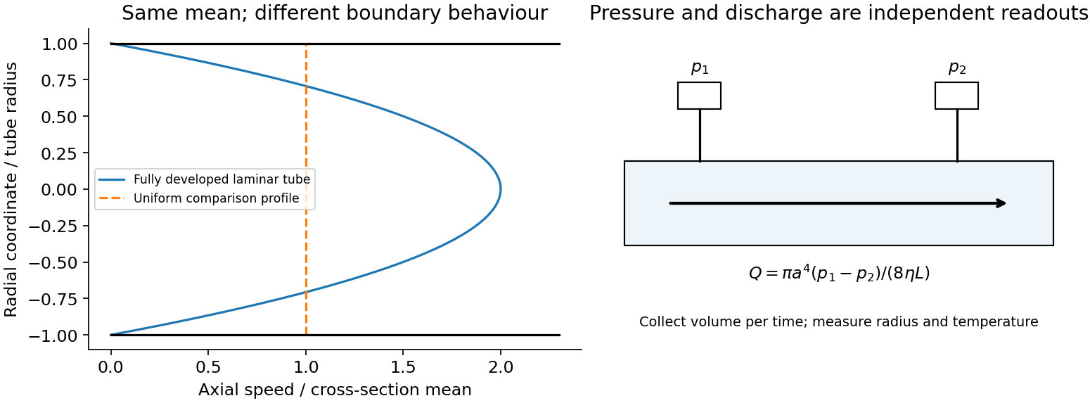
In a long straight circular tube, steady fully developed laminar flow hasThis Hagen-Poiseuille equation follows by balancing the axial pressure gradient with viscous shear and setting $v_z(a)=0$. The parabolic profile, the fourth-power radius sensitivity and the pumping power $\Delta pQ$ are experimentally distinct consequences. Entrance regions, rough walls, non-Newtonian response or a changing temperature require additional modelling.

The Reynolds number $\mathrm{Re}=\rho UL/\eta$ compares inertia with viscosity. Small values favor creeping-flow balances; high values permit thin boundary layers, separation and turbulence, although transition depends on geometry and perturbations, not one universal critical number. At high Reynolds number an outer flow can be approximately inviscid while near-wall viscosity still determines drag. This resolves why a zero-drag ideal potential-flow model cannot predict the resistance of an ordinary moving body. In turbulent flow, fluctuating Reynolds stresses redistribute momentum and increase the required pressure drop; averaging the equations introduces closure requirements.

A controlled tube experiment measures pressure difference and collected volume per time while changing forcing. Use tracers or a velocity probe to test profile shape, allow sufficient entrance length, and monitor radius and temperature independently. Repeat with reversed flow and at several rates to test offsets and linearity. Dye mixing alone does not measure viscosity or establish a fully developed velocity profile. The original figure below separates a specified laminar velocity profile from an independent pressure/discharge measurement.