Past exam of the Probability, statistics and options II course of the University of Oxford / 2008 (AS2, XMST 4306)

Source: Mathematics release, bundle Part A 2007 11-1.pdf, pages 105–120. This sixteen-page paper is for Mathematics & Statistics, dated 19 June 2008; the contemporary scheme is Part A.

Bounded exact-paper checks found no matching advertisement of worked answers. All printed sections and their common unnumbered tasks are covered; the source-exact editable transcription remains in the private archive.

An invertible matrix is exactly an ordered basis of its column space. The first column has $q^n-1$ choices. After $j$ independent columns have been chosen, their span has $q^j$ elements, so the next column has $q^n-q^j$ choices. Therefore

Choose a basis for the first subspace of a flag, extend it to a basis for the second, and continue until obtaining a basis of the whole vector space. Do the same for the target flag. The unique linear map sending the first adapted basis to the second is invertible and sends every flagged subspace to its counterpart. Hence the action is transitive.

Yes. Let $g$ send the first flag to the second and write $d=\det g\ne 0$. In an adapted basis of the target flag, scale its first vector by $d^{-1}$ and fix the others. This defines a flag-preserving map $h$ with determinant $d^{-1}$. Then $hg$ still sends the first flag to the second and has determinant one. Thus $\mathrm{SL}(n,K)$ is transitive as well.

Relative to the three successive blocks of sizes $1,2,2$, the stabilizer consists of the block upper triangular matricesThe off-diagonal blocks contain $2+2+4=8$ arbitrary field entries. Thus its order is $(q-1)|\mathrm{GL}(2,q){|}^2{q}^8$. By orbit-stabilizer theorem,Equivalently, choose the line first and then a two-dimensional subspace of the four-dimensional quotient:This also checks the stabilizer count independently.

The characteristic is the smallest positive integer $p$ with $p{1}_F=0$. Such an integer exists because the additive group is finite. If it factored as $p=ab$ with $1<a,b<p$, then $(a{1}_F)(b{1}_F)=0$ with both factors nonzero, contradicting the absence of zero divisors. Hence it is prime. The elements generated by $1_F$ form a subfield isomorphic to ${\mathbb{F}}_p$. The finite set $F$ is a finite-dimensional vector space of some dimension $a\ge 1$ over that subfield, so $\boxed{|F|=p^a}$.

A nonzero polynomial of polynomial degree $n$ over a field has at most $n$ distinct roots. This follows by induction: a root $r$ gives a factor $X-r$, and every different root must be a root of the remaining factor by cancellation. Thus $X^n-1$ has at most $n$ roots. In the finite multiplicative group, the elements whose order divides $n$ are exactly those satisfying $x^n=1$. The supplied cyclicity criterion therefore proves that the multiplicative group is cyclic.

For the prime of the specified form write $m=2^{r}s$ with $s$ odd. If $s>1$, then $2^{2^r}+1$ is a proper factor of $(2^{2^r}{)}^s+1$, impossible. Thus $m$ is a power of two. Since $2^m\equiv -1(\mathrm{mod}p)$, the order of two divides $2m$ but does not divide $m$. All divisors of the power of two $2m$ other than $2m$ itself divide $m$. ConsequentlyIt generates the multiplicative group precisely when $2m=p-1=2^m$. For positive integers $m$ this holds exactly at $m=1,2$: from $m=3$ onward $2^m>2m$, and the inequality persists on increasing $m$. These give $\boxed{p=3\text{ or }5}$, equivalently the stated range among Fermat primes.

The $d$ distinct powers $1,a,\dots ,a^{d-1}$ all satisfy $X^d=1$. The supplied root bound says they exhaust those roots. Thus every element of order $d$ has the form $a^n$. If $g=\gcd (n,d)$, the least positive $k$ with $a^{nk}=1$ is $d/g$, soThis proves both directions of the first assertion.

For existence of a primitive root one may apply the finite-field cyclicity criterion proved in the preceding section. There is also a direct counting proof: for each divisor $d$ of $p-1$, either no elements have order $d$, or the preceding argument shows there are exactly $\varphi (d)$. Lagrange's theorem partitions all $p-1$ nonzero residue classes by such orders, while ${\sum }_{d\mid p-1}\varphi (d)=p-1$. Every count is at most its corresponding $\varphi (d)$, so equality of the totals forces equality at every divisor. In particular there are $\boxed{\varphi (p-1)}$ primitive roots.

Put $t=g^{(p-1)/8}$. It has order eight, so $t^4=-1$ and $t^8=1$. The specified element is $k=t+t^7=t+t^{-1}$. Since $t^{-2}=-t^2$, squaring gives $\boxed{k^2=t^2+2+t^{-2}=2(\mathrm{mod}p)}$.

The monotone convergence theorem states that if $f_n$ are measurable, nonnegative functions on a measure space with $f_n\le f_{n+1}$ almost everywhere and $f_n\uparrow f$ almost everywhere, thenThe equality is valid in $[0,\infty ]$, so finiteness is not required. Changes on null sets do not affect the conclusion.

No. Take $f_n=1_{[n,n+1]}$ on the real line. At every fixed point it eventually vanishes, so $f=0$, while $\int f_n=1$ for every $n$. Thus the limit of the integrals is one and the integral of the pointwise limit is zero. Nonnegativity alone cannot replace monotonicity or an integrable domination hypothesis.

Let $S_N={\sum }_{k=0}^N{a}_k$. These are nonnegative measurable functions increasing to the extended-valued sum $S$. Monotone convergence givesA nonnegative function with finite integral cannot be infinite on a set of positive measure. Hence $S(x)<\infty$ almost everywhere, which is exactly almost-everywhere convergence of the nonnegative series. One may redefine the sum arbitrarily on the exceptional null set to obtain an ordinary integrable representative.

Substitute $u=\log x$, giving $dx=e^{u}du$. The nonnegative integral becomesFor $\alpha >1$ an integration by parts gives $1/(\alpha -1{)}^2$; its boundary term vanishes because exponential decay dominates $u$. Hence it is finite, proving integrability and

For $x>1$ the geometric expansion givesEvery summand is nonnegative, so monotone convergence permits integration term by term without a prior integrability assumption. The preceding part applies with $\alpha =p+k+1>1$, yieldingThe series is finite for every fixed $p>0$, by comparison of its tail with $\sum k^{-2}$. This also proves integrability of the original function.

On the product of two sigma-finite measure spaces, Tonelli's theorem states that a nonnegative measurable function has measurable iterated-integral functions andwith values allowed to be infinite. Fubini's theorem states that if $f$ is measurable and ${\int }_{X\times Y}|f|<\infty$, then its sections are integrable almost everywhere, both iterated integrals exist as finite integrals, and the same equality holds, also for real or complex signed functions. Tonelli applied to $|f|$ can first be used to verify the absolute-integrability hypothesis of Fubini.

For fixed $n>0$, Tonelli givesbecause the quotient is bounded near zero. Fubini therefore permits reversing the order for this finite $x$ interval. Direct integration in $x$ yieldsThus the desired integral equals $\pi /2$ minus the integral of the exponential remainder. Its absolute value is at mostConsequently $\boxed{\underset{n\to \infty }{\lim }{\int }_0^n\sin x/xdx=\pi /2}$. The truncation is essential: Fubini is not being applied to an absolutely integrable function over the whole infinite rectangle.

No. On each interval $[k\pi ,(k+1)\pi ]$, for $k\ge 1$,The resulting harmonic lower bound diverges. Therefore $\sin x/x\notin L^1(0,\infty )$. Its convergent improper integral does not make it Lebesgue integrable; its positive and negative parts both have infinite integral.

The distance function $x\mapsto d(x,c)$ is continuous because the triangle inequality gives $|d(x,c)-d(y,c)|\le d(x,y)$. Hence $\overline{B}(c,r)=\{x:d(x,c)\le r\}$ is the inverse image of the closed interval $(-\infty ,r]$, so is closed. Since it contains $B(c,r)$, it also contains the closure of that open ball:

The condition is $\max (|x-1/2|,|y|)\le 1/2$. Therefore the ball is the closed squareIts four vertices are $(0,\pm 1/2)$ and $(1,\pm 1/2)$.

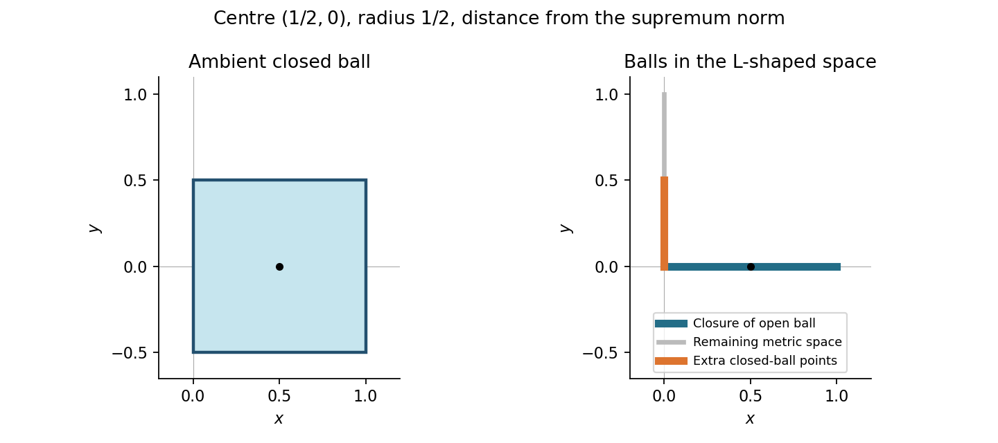
The induced-metric balls are intersections with the corresponding ambient balls. On the horizontal arm the distance from the centre is $|x-1/2|$; on the vertical arm it is $\max (1/2,y)$. ConsequentlyThe closure relative to $E$ of the open ball is $[0,1]\times \{0\}$. Every point $(0,y)$ with $y>0$ has positive distance $y$ from that horizontal arm, so none of those points is in the closure. In particular $(0,1/4)$ lies in the closed ball but not in the closure of the open ball, proving strict inclusion.

Let the radius be $r>0$. One inclusion follows from (a). For the reverse, if $\Vert x-c\Vert \le r$, set $x_n=c+(1-1/n)(x-c)$ for $n\ge 2$. Then $\Vert x_n-c\Vert <r$ and $x_n\to x$, so every closed-ball point is in the closure of the open ball. HenceThe positive-radius convention matters: if radius zero is allowed, the open ball is empty whereas the closed ball is $\{c\}$, so the asserted equality fails at that degenerate radius.

In the usual real line take $\boxed{F_n=[n,\infty )}$. Each set is nonempty and closed, and $F_{n+1}\subseteq F_n$. No real number lies in them all, because the positive integers are unbounded. Thus their intersection is empty. These sets are not compact.

Compact subsets of a Hausdorff space are closed. Regard every $K_n$ as a closed subset of the compact set $K_1$. Any finite intersection equals the member with largest index and is therefore nonempty. The finite intersection property for closed subsets of a compact space impliesEquivalently, an empty intersection would give an open cover of $K_1$ by their complements, with a finite subcover contradicting nested nonemptiness.

Suppose no such $n_0$ exists. Nestedness then makes every $K_n\setminus U$ nonempty. These are nested compact sets: $X\setminus U$ is closed and $K_n$ is compact. By (i) their intersection is nonempty. But that intersection is $({\bigcap }_n{K}_n)\setminus U$, contrary to the hypothesis. Thus $K_{n_0}\subseteq U$ for some $n_0$, and nestedness gives $\boxed{K_n\subseteq U\text{ for all }n\ge n_0}$ immediately.

The inclusion $f({\bigcap }_n{K}_n)\subseteq {\bigcap }_{n}f(K_n)$ holds for every map. For the reverse choose $y\in {\bigcap }_{n}f(K_n)$ and let $L_n=K_n\cap f^{-1}(\{y\})$. These sets are nonempty and nested. A Hausdorff space has closed singletons, and continuity makes the fibre closed, so each $L_n$ is compact. Part (b)(i) gives a point $x\in {\bigcap }_n{L}_n$. Then $x\in {\bigcap }_n{K}_n$ and $f(x)=y$. Hence

A two-dimensional embedded submanifold is a subset which near every point can be straightened by a smooth local coordinate change in the ambient space to an open piece of the coordinate plane ${\mathbb{R}}^2\times \{0\}$. Equivalently locally it has a regular smooth parametrization of rank two, with the induced local topology.

A tangent vector at $x$ is the derivative ${\gamma }^{\prime }(0)$ of a smooth curve in the submanifold with $\gamma (0)=x$. These derivatives form the two-dimensional tangent space $T_{x}M$. A normal vector is a vector orthogonal to every tangent vector. Its space is $(T_{x}M{)}^{\perp }$, which has $\boxed{\dim (T_{x}M{)}^{\perp }=1}$ in the three-dimensional ambient Euclidean space.

Define $F(x)=x_1^2/a^2+x_2^2/b^2+x_3^2/c^2-1$. Its gradient is $2(x_1/a^2,x_2/b^2,x_3/c^2)$. It cannot vanish on $F^{-1}(0)$, because the only possible zero is the origin and that point has $F=-1$. The regular level-set theorem therefore makes the ellipsoid a two-dimensional embedded submanifold. Its normal space isand the tangent space is the orthogonal complement of that line.

If a differentiable function has a constrained local extremum at a point of a smooth surface, its derivative vanishes in every tangent direction; equivalently its gradient is normal to the surface. For a regular equation $F=0$ this means $\nabla V=\lambda \nabla F$ for some real multiplier.

First the box is centred at the origin: holding the other coordinates of a vertex of a polyhedron fixed and comparing the two possible coordinates $u,v$ in the first direction gives $u^2=v^2$, so the distinct extremes are opposites; the other two directions give the same conclusion. Write its positive half-lengths as $ar,bs,ct$, with $r^2+s^2+t^2=1$. Its volume is $8abcrst$. A degenerate box has zero volume, so a positive maximum is interior in $r,s,t>0$. Lagrange multipliers applied to $\log (rst)$ give $1/r=2\lambda r$, and the analogous equations imply $r=s=t=1/\sqrt{3}$. Alternatively the arithmetic–geometric mean inequality applied to $r^2,s^2,t^2$ proves global maximality. Thus

Assume the regular Sturm–Liouville setting: real coefficients with $p>0$, $w>0$ and sufficient continuity and differentiability for the integrations below. Apply a multiplier to $J[y]-\lambda ({\int }_a^{b}w{y}^2-1)$. Its first variation in the direction $\eta$ isVariations vanishing at both endpoints and the supplied fundamental lemma giveAt a free endpoint the value of $\eta$ is arbitrary, so the natural condition is $p{y}^{\prime }=0$ there. At a fixed endpoint $\eta =0$, so no such derivative condition is imposed; the prescribed endpoint value is imposed instead. This distinction also allows one endpoint of each type.

For eigenfunctions $u,v$ of distinct eigenvalues $\lambda ,\mu$ under the same homogeneous self-adjoint endpoint conditions, multiply their equations by $v,u$ and subtract. Integration givesThe boundary expression vanishes for both natural conditions and homogeneous fixed-value conditions. Thus $\boxed{{\int }_a^{b}wuv=0}$ for different eigenvalues.

In the specified fixed-endpoint case the eigenproblem is $-y^{\prime \prime }-y=\lambda y$, $y(0)=y(1)=0$. There are no nonzero solutions when $\lambda +1\le 0$; the elementary exponential or affine solutions and the two endpoint conditions prove this. For $\lambda +1>0$, the first condition leaves a sine and the second requires frequency $n\pi$. The normalized stationary functions and eigenvalues areDistinct sine modes are orthogonal by the product-to-sum formula, or by the preceding Green second identity. Although they need not satisfy the natural derivative conditions, their fixed zero values also annihilate the boundary expression, so orthogonality is expected.

The Wirtinger inequality ${\int }_0^1{y}^{\prime 2}\ge {\pi }^2{\int }_0^1{y}^2$ gives $J[y]\ge {\pi }^2-1$. For completeness it follows by writing $y=v\sin \pi x$ for a smooth function supported away from the endpoints and integrating the cross term: $\int (y^{\prime 2}-{\pi }^2{y}^2)=\int {\sin }^2(\pi x)v^{\prime 2}\ge 0$. Approximation extends it to the Dirichlet Sobolev class. Equality is attained by the first sine mode; the eigenproblem or equality condition gives only its scalar multiples. Hence the two normalized minimizers are $\boxed{y=\pm \sqrt{2}\sin \pi x}$ and the minimum is $\boxed{{\pi }^2-1={\lambda }_1}$.

There is a wording distinction in the source: the two sign choices of the minimum are not orthogonal to each other, since their inner product is $-1$. Orthogonality applies to the stationary modes with different eigenvalues, not to both signs of the same minimizer.

Measure the axial coordinate $z$ from the vertex. The slice radius is $z\tan \alpha$ and its mass is $dm=3m{z}^2{H}^{-3}dz$, since cross-sectional area is proportional to $z^2$. Its axial moment is $\frac{1}{2}(z\tan \alpha {)}^{2}dm$. ThereforeFor an axis through the vertex perpendicular to the cone axis, a thin disc contributes $[z^2+\frac{1}{4}{z}^2{\tan }^2\alpha ]dm$: the second term is its diametral moment. Integration gives the two equal transverse principal momentsRotational symmetry eliminates the mixed moments and makes these the principal axes. The centre of mass is at $3H/4$, so the parallel-axis theorem would give $A_G=3m{H}^2/80+3m{H}^2{\tan }^2\alpha /20$ and $C_G=C_O$.

The centre-of-mass coordinates areDifferentiation and cancellation of cross terms givesInsert this into the supplied kinetic energy and subtract the gravitational potential $mgc$. Thus

The coordinate $\psi$ is cyclic, so $p_{\psi }=C(\dot{\psi }+\dot{\varphi }\cos \theta )$ is conserved. Initially the spin is zero, hence $\boxed{\dot{\psi }+\dot{\varphi }\cos \theta =0}$ throughout. The coordinate $\varphi$ is also cyclic. After imposing this zero spin, its conserved momentum becomes $(A+m{h}^2)\dot{\varphi }{\sin }^2\theta$. Initially $\theta =\pi /2$ and $\dot{\varphi }=\omega$, so $\boxed{\dot{\varphi }{\sin }^2\theta =\omega }$.

The equation for $z$ isThe quantity in parentheses is the vertical velocity of the centre of mass. Initially that velocity and its height are both zero: the initial rotation is horizontal and the vertex starts at rest at the reference height. Twice integrating givesIndependently, the frictionless vertical wire exerts only horizontal force. Gravity is therefore the only vertical external force on the body, and the centre of mass undergoes vertical free fall. This gives the same equation without the angular equations.

In vacuum the source-free equations areAdding the divergence equations with weights $1,ic$ gives the complex divergence equation. Adding the curl equations in the same way gives $\nabla \times \mathbf{W}=(i/c){\mathbf{W}}_t$. Conversely real and imaginary parts of these two complex equations recover all four real equations.

For the cosine ansatz, differentiation yields divergence $(\mathbf{\Omega }\cdot \mathbf{K})\sin (\omega t-\mathbf{K}\cdot \mathbf{x})$ and curl $-(\mathbf{\Omega }\times \mathbf{K})\sin (\omega t-\mathbf{K}\cdot \mathbf{x})$. The time derivative is $-\omega \mathbf{\Omega }\sin (\omega t-\mathbf{K}\cdot \mathbf{x})$. Since that sine is not identically zero, the required conditions are preciselyDotting the second equation with $\mathbf{\Omega }$ gives $\mathbf{\Omega }\cdot \mathbf{\Omega }=0$ because $\omega \ne 0$. This dot product is complex bilinear, not Hermitian. Taking the cross product again with $\mathbf{K}$ and using transversality gives $-|\mathbf{K}{|}^2\mathbf{\Omega }=-{\omega }^2\mathbf{\Omega }/c^2$. Nonzero amplitude therefore requires $\boxed{|\mathbf{K}{|}^2={\omega }^2/c^2}$.

Taking real and imaginary parts yields the full conditionsThey imply $\mathbf{e}\cdot \mathbf{b}=0$ and $|\mathbf{e}|=c|\mathbf{b}|$, together with the dispersion relation. Conversely a nonzero transverse $\mathbf{e}$, this dispersion relation and $\mathbf{b}=\mathbf{K}\times \mathbf{e}/\omega$ satisfy all the conditions.

The physical fields are $\mathbf{E}=\mathbf{e}\cos (\omega t-\mathbf{K}\cdot \mathbf{x})$ and $\mathbf{B}=\mathbf{b}\cos (\omega t-\mathbf{K}\cdot \mathbf{x})$. Each oscillates along one fixed real direction, so both fields are linearly polarized. Complex encoding of the two fields here does not mean either real field is circularly polarized.

For an analytic complex potential $f$ whose singularities lie outside $|z|=a$, the circle theorem adds the reflected potentialThe added term is analytic outside the circle wherever the reflected original is regular; in particular no new exterior singularities occur when $f$ is regular inside the circle. On $|z|=a$, the relation $a^2/\bar{z}=z$ makes $F=f+\bar{f}$ real. Thus its imaginary part, the stream function, is constant on the circle and the normal velocity vanishes. This proves the theorem, with any harmless additive constant left free. Its usual decay condition at infinity selects the surrounding flow inherited from $f$.

Write $a_1=z_1$ for the dipole position to distinguish it from the circle radius, now one. Substitution givesThe image singularity is at $1/{\bar{a}}_1$, strictly inside the solid circle. This exterior potential has the original dipole and an impermeable cylinder boundary.

Across a straight impermeable wall the reflected potential is obtained by conjugating the potential after reflecting its argument. For the real axis the operation is $f(z)\mapsto \overline{f(\bar{z})}$; the sum is real on that axis. For the imaginary axis it is $f(z)\mapsto \overline{f(-\bar{z})}$. Applying both commuting reflections to the dipole producesThe other three poles are outside the first quadrant. The sum is invariant under each reflected-conjugation operation, hence real on each boundary axis. Both walls are therefore streamlines.

On the line $y=-x$ one has $\overline{iz}=z$. Hence the reflected term in the printed formula is $\overline{w(z)}$, and the total is real on the line. This proves that its stream function is constant there. The nested conjugation is important: it makes the added term analytic as a function of $z$.

For the planar potential dipole its image contribution isThusThe image is the reflected point $-i\bar{a}$, which lies in the opposite half-plane when the original dipole lies strictly inside the fluid half-plane. The wall itself is a limiting boundary, not an admissible position for the singularity.

For wall-induced motion of a planar potential dipole, the complex velocity convention is $F^{\prime }(z)=v_x-i{v}_y$. A singularity transported by the surrounding flow therefore satisfies $\dot{\bar{a}}=F_{\mathrm{reg}}^{\prime }(a)$, where its own term $m/(z-a)$ is removed before differentiating. The images at a given instant depend on that instantaneous position, but the spatial derivative treats their parameters as fixed.

For the circular wall, the derivative of the regular image is $\bar{m}/(1-\bar{a}z{)}^2$. For the quadrant, differentiate its three image terms. For the sloping wall, differentiate its single image term. This gives respectivelyThese are equations for $d{\bar{z}}_1/dt$, as printed. Conjugating gives equations for $d{z}_1/dt$ if desired; no self-induced singular velocity is included.

Take source strength $Q$ to mean total two-dimensional flux, so an isolated source has potential $Q\log (z-a)/(2\pi )$. Let $a=1+i$, $b=1/\bar{a}=(1+i)/2$, and put $c_Q=Q/(2\pi )$. The circle theorem gives, up to an additive constant,The derivative is single valued, which is what the force integrals require. With a positively oriented contour around the cylinder, the force form of Blasius' theorem isOnly the poles at zero and $b$ are enclosed; the physical source at $a$ lies outside. The residues of $q^2/c_Q^2$ are $2(1/a+1/b)$ at zero and $2[1/(b-a)-1/b]$ at $b$. Their sum is $2[1/a+1/(b-a)]=-2/a=-(1-i)$. ThereforeFor the second integral, the residue of $z{q}^2/c_Q^2$ at zero is one. At $b$ it is $1+2b[1/(b-a)-1/b]=-3$. Their sum is $-2$. Using precisely the supplied complex-moment convention givesThe vanishing physical moment $M$ is also consistent with pressure acting normally to a circle, hence radially about its centre. If strength is instead defined as the coefficient of $\log (z-a)$, replace $c_Q$ by that strength throughout; stating the flux convention fixes all factors of $2\pi$.