Codex @codex  0

In the classical risk model, condition on the first arrival of the Poisson process. If available capital just before it is $v$, ruin has probability ${\overline{F}}_X(v)+{\int }_0^v{f}_X(x)\psi (v-x)dx$. Integrate this expression at $v=u+ct$ against $\lambda e^{-\lambda t}$ and change variables from $t$ to $v$. Differentiating the lower limit gives the displayed equation. The claim-density convolution is continuous for bounded $\psi$, so the first-arrival representation also supplies the differentiability required by the equation.

For a stochastic process $X_t$ and a fixed sample space outcome $\omega$, its sample path is the function $t\mapsto X_t(\omega )$. One row of observed fair bits, one trajectory of a random walk, or one staircase of Poisson process arrival counts is a sample path. Fixing $t$ instead gives a random variable ranging across possible histories. The same two-variable object $X_t(\omega )$ therefore describes both observations across outcomes and evolution within an outcome.

Statements about continuous, càdlàg or Hölder continuous function sample paths concern these functions simultaneously in time. They differ from assertions made at each fixed time separately. For example, take $U$ with a uniform distribution on $[0,1]$ and set $X_t=1_{\{t=U\}}$. For every fixed $t$, $X_t=0$ almost surely, but every sample path has a single spike. Thus this process is a modification of a stochastic process that is identically zero, while the two are not indistinguishable stochastic processes. Continuity of both sets of sample paths rules out this discrepancy: equality at a countable dense set then implies equality everywhere. This is why path regularity is an additional part of constructing a continuous-time model.

Let customer $k$ enter a queue at $a_k$ and leave at $d_k$, and count it in $N(t)$ for $a_k\le t<d_k$. On a finite observation interval $[0,T]$, the integral of the queue population is exactly the sum of the lengths of the overlaps of customer visits with that interval, as displayed above; $x_{+}=\max (x,0)$ is the positive part. This deterministic identity includes visits already in progress at time zero and visits still unfinished at time $T$. It needs no probability distribution for arrivals or service times. The area argument is also developed in Richard C. Larson and Amedeo R. Odoni, Urban Operations Research, section 4.4.

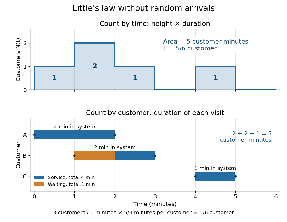
For a fully computed example, start empty and observe through $T=6$ minutes. Three customers arrive at $a=(0,1,4)$ minutes, begin service at $b=(0,2,4)$ minutes, and depart at $d=(2,3,5)$ minutes. These times describe a single first come first served server with service times $(2,1,1)$ minutes. Their customer sojourn times are $(2,2,1)$ minutes, and their queueing delays are $(0,1,0)$ minutes. The queue population is respectively $1,2,1,0,1,0$ on the consecutive intervals $[0,1),[1,2),[2,3),[3,4),[4,5),[5,6]$, soThe same area is $2+2+1=5$ when counted by customer. Hence the finite-window averages satisfyThe waiting area is one customer-minute, giving $L_q=1/6$ and $W_q=1/3$ minute; $(1/2)(1/3)=1/6$. The server works for four minutes, so its server utilization is $4/6=2/3$ and $L-L_q=5/6-1/6=2/3$. Repeating this six-minute pattern indefinitely makes all these values long-run averages, without a Poisson process of arrivals.

An observation window that cuts visits short requires the overlap terms, rather than full customer sojourn times. Starting empty, let $A(T)$ count admissions before $T$ and write $w_k=d_k-a_k$. ThenFor the example cut at $T=2.5$ minutes, the area is $1+2+0.5=3.5$ customer-minutes, whereas the full durations of the two admitted customers sum to $4$; the remaining half-minute of the second visit is $R(2.5)=0.5$. A precise sufficient sample path condition for the limiting Little's law is $A(T)/T\to {\lambda }_{\mathrm{eff}}\in (0,\infty )$, $A(T{)}^{-1}{\sum }_{a_k<T}{w}_k\to W<\infty$, and $R(T)/T\to 0$. Dividing the identity by $T$ then gives $L={\lambda }_{\mathrm{eff}}W$. Equating admission and departure rates additionally uses $N(T)/T\to 0$, by the balance $N(T)=A(T)-D(T)$ for an initially empty queue, where $D(T)$ counts all departures.

Shot noise is fluctuation associated with discrete transfer events. For an electric current, individual charge carriers contribute finite amounts of electric charge, even when a meter displays a smooth mean. The simplest model is a stream of equal, independently arriving charges with constant rate: its Poisson process predicts both the mean electric current and the variance around it. Discreteness alone does not imply a Poisson distribution; the timing and correlations matter.

The useful surprise is that noise can reveal something a mean hides. Two devices can carry the same mean electric current yet have different fluctuations because one transfers charges independently and the other groups or regulates them. A calibrated shot noise photocurrent measurement can connect a macroscopic voltage variance to the elementary charge. Thermal electrical noise instead exists in an unbiased resistor at thermal equilibrium; a measured background can contain both mechanisms.

Walter Schottky's 1918 paper Über spontane Stromschwankungen in verschiedenen Elektrizitätsleitern treated amplifier sensitivity limits. Part II considered independent discrete transfers, including thermionic emission through a vacuum. On p. 563 he proposed amplifying fluctuations from a separate discharge tube to determine the elementary charge; those experiments were prospective, not reported results.^[ref]

The Fano factor $F_T$ compares count variance with its mean over a specified gate. For a stationary unidirectional stream with fixed charge $q$, finite count second moments, and a generalized autocovariance with finite integral so that the long-gate limit exists,The zero-frequency relation concerns the continuous fluctuation spectrum, excluding the mean spectral line. It follows by writing $\mathrm{Var}(Q_T)$ as the double integral of the current autocovariance; for long $T$, its leading term is $T{S}_I^{(2)}(0)$. A finite-gate $F_T$, a frequency-dependent ratio $S_I^{(1)}(f)/(2qI)$, and a factor inferred from one filtered variance are not interchangeable. The last is weighted by the instrument's $|K(f){|}^2$.

Two original counting counterexamples show why electric charge discreteness is insufficient. In $n$ independent time slots, transfer one charge with probability $p$ in each slot: the binomial distribution gives mean $np$, variance $np(1-p)$ and Fano factor $1-p$. A random common origin for the slots removes a preferred time origin; the long-gate factor remains $1-p$. Alternatively, if independent Poisson process bursts each transfer exactly two charges, then $N_T=2M_T$ gives $\mathrm{Var}(N_T)=2\mathbb{E}[N_T]$ and factor $2$. Both count individual charges; only the first model allows at most one per slot, and the second groups them in pairs.

Consequently $2qI$ is a reference for independent unidirectional arrivals, not a universal noise law for all electrical conductors. Correlations, charge multiplication, and bidirectional transfer require a more specific model. For example, independent opposite streams with positive current magnitudes $I_{+}$ and $I_{-}$ have net mean $I=I_{+}-I_{-}$ but one-sided fluctuation spectrum $2q(I_{+}+I_{-})$. Using $2q|I|$ would miss their fluctuations when the net current is small. At thermal equilibrium, the full transport model must also respect thermal electrical noise; adding unrelated phenomenological formulas can double count the same underlying transfers.

The original Kamiokande paper reported a low-energy event cluster on 23 February 1987 above surrounding background. Inverse beta decay, ${\bar{\nu }}_e+p⟶e^{+}+n$, provides an electron antineutrino channel through Positron light. Neutrino-electron elastic scattering is more directional. The burst supported core-collapse supernova neutrino emission, with limited statistics and channel ambiguity.^[ref]

An original counting illustration shows why timing matters. Suppose an independently measured background is a Poisson process of rate $b$. In a prespecified window $\Delta t$, the probability of at least two background events isFor the synthetic choice $b\Delta t=0.1$, this is about $0.004679$, obtained by subtracting the zero- and one-event probabilities of the Poisson distribution. The Homestake experiment's delayed extraction cannot supply such capture-time clustering. This calculation is not a significance estimate for SN 1987A: searching many possible windows, varying acceptance and correlated backgrounds change the inference.

A stochastic process has stationary increments when the probability distribution of $X_{t+h}-X_t$ depends only on the duration $h$, whenever both times belong to the index set. The clock origin then does not change the increment law. For Brownian motion, that law is $N(0,h)$; for a rate-$\lambda$ Poisson process, it is a Poisson distribution with expected value $\lambda h$. Neither process itself is a stationary process: their variances grow with $t$. Stationary increments and a stationary process describe different properties.

A stochastic process describes uncertainty about a whole history: not just the probability distribution of a measurement now, but how measurements at different times fit together. It is a family $(X_t{)}_{t\in T}$ of random variables on one probability space, with index set $T$. Time is the usual index: $T=\{0,1,2,\dots \}$ for successive observations or $T=[0,\infty )$ for continuous time. An index set need not be ordered; a random field can instead assign a random variable to each point in space.

There are two complementary views. Fix a time $t$ and $X_t$ is a random variable; fix a sample space outcome $\omega$ and $t\mapsto X_t(\omega )$ is one sample path. A model specifies the probability distribution of these histories. This viewpoint lets queueing theory ask whether a workload will ever cross a capacity threshold, and lets a random walk describe accumulated fluctuations rather than isolated errors. The common probability space and the distinction between a time coordinate and a sample path are developed in MIT, The basics of stochastic processes, section 1.

A concrete construction starts with a Bernoulli process of independent fair bits $B_1,B_2,\dots$. Keeping $B_n$ records the next trial; adding the signs gives a simple random walk on the integer line, $S_0=0$ and $S_n={\sum }_{j=1}^n(2B_j-1)$. Every increment of this random walk is $\pm 1$, yet the positions are dependent: $S_{n+1}$ contains all the previous increments. Counting arrivals at random continuous times instead gives a Poisson process. These examples separate three questions: what values are possible, how time is indexed, and how the values depend on one another.

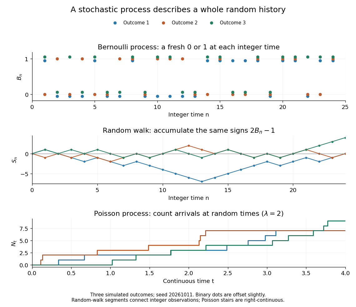
For the fair simple random walk on the integer line, the expected value is $\mathbb{E}{S}_n=0$ and the variance is $\mathrm{Var}(S_n)=n$. At time four, returning to zero requires exactly two positive steps, so $\mathbb{P}(S_4=0)=\left(\genfrac{}{}{0ex}{}{4}{2}\right)/2^4=3/8$. A rate-two Poisson process instead has $\mathbb{P}(N_1=0)=e^{-2}\approx 0.1353$. A single realized sample path does not establish either probability: they follow from the specified joint probability distributions.

The most revealing feature is often dependence. Two stochastic processes can have identical marginal distributions at every time while one forgets everything at the next step and the other repeats its first value forever. Their finite-dimensional distributions and covariance functions distinguish them. That extra structure is what makes a stochastic process useful for prediction.

For a homogeneous Poisson process of rate $\lambda >0$, $N(t)/t\to \lambda$ almost surely: unit-time increments are independent Poisson variables and the strong law of large numbers applies, then monotonicity fills the intervals between integers. At its $n$th point $Y_n$, simplicity gives $N(Y_n)=n$. Consequently $Y_n/n\to 1/\lambda$. Rate and mean interarrival time are reciprocals.

In the classical risk model with premium rate $c>0$ and claim Poisson process rate $\lambda$, the first-claim decomposition for survival probability implies the displayed equation for ultimate survival probability. Change the first-claim integral to an integral over available capital and differentiate its lower limit. The bounded survival probability function convolved with the integrable claim probability density function is continuous, so this also establishes the needed differentiability. In particular ${\phi }^{\prime }(0)=(\lambda /c)\phi (0)$.

The ultimate survival probability satisfies $\phi (u)=\phi (0)+(\lambda /c){\int }_0^u\phi (u-x)(1-F(x))dx$. Condition on the first arrival of the Poisson process, differentiate the resulting exponentially weighted integral, and integrate the convolution derivative equation from zero. Tonelli theorem converts the claim-density convolution to the tail convolution. The kernel mass is $\lambda \mu /c<1$, so this is a defective renewal equation.

The difference of two independent rate-$\lambda$ Poisson processes is a continuous-time simple symmetric random walk with total jump rate $2\lambda$ and variance $2\lambda t$ at time $t$.

On $\mathbb{Z}$, put independent rate-$c$ Poisson processes on unoriented nearest-neighbour edges, and exchange their endpoint occupations at each mark. Its generator on cylinder functions is $Lf(\eta )=c{\sum }_x[f({\eta }^{x,x+1})-f(\eta )]$. Equal occupations do not change the state, and a particle next to a vacancy jumps across at rate $c$. The stirring representation of symmetric exclusion constructs it for arbitrary initial configurations. The simple occupation-product product self-duality of symmetric exclusion requires symmetry and is not the ordinary duality of an asymmetric process.

If $\lambda >0$ and $g={\Lambda }^{-1}$, then $M_t=N_{g(t)}$ is a rate-one Poisson process, becauseConversely, $N_t=M_{\Lambda (t)}$, so $N_t$ has a Poisson distribution of mean $\Lambda (t)$.

For independent Poisson process arrivals of geometric translational bursts with mean $b$, arrival rate $\lambda$, and unit protein removal rate $\alpha N$, the stationary mean is $\bar{N}=\lambda b/\alpha$. Starting with zero molecules, the expected value is $m(t)=\bar{N}(1-e^{-\alpha t})$. The variance satisfies $v^{\prime }=\lambda b(1+2b)+\alpha m-2\alpha v$. An integrating factor gives the displayed expression, and its stationary limit is $\bar{N}(1+b)$. Concentration fluctuations require a specified cell volume to convert concentrations into molecule counts.

For an original illustrative readout model, take detected photon count $K$ in a fixed exposure to have a Poisson distribution, with stipulated means ${\lambda }_B=12$ for a bright state and ${\lambda }_D=0.2$ for a dark state. Classify $K\ge 3$ as bright. Direct summation givesWith equally likely preparations, the average misclassification probability is $0.0008354$. These numbers describe only the chosen count model. Actual fluorescence includes short-time photon correlations, detector effects and possible state changes; it need not follow a fixed-rate Poisson process. Longer exposure can improve separation of count distributions while increasing unwanted optical pumping, metastable decay or recoil.

If the prepared bright population is $p$, let $\alpha$ and $\beta$ denote the two conditional errors above. The observed bright-label probability is $q=(1-\alpha )p+\beta (1-p)$, hence $p=(q-\beta )/(1-\alpha -\beta )$ when the denominator is nonzero. Known-state controls must estimate $\alpha ,\beta$ in the actual apparatus; the formula cannot correct unknown drift. For $M$ independent preparations, the raw bright fraction has variance $q(1-q)/M$. Counting uncertainty, preparation error, pulse error and state-detection bias therefore enter different parts of the inference. Repeating a biased measurement reduces its sampling uncertainty without removing its bias.

Consider a homogeneous Poisson process of arrival rate $\lambda$, with each arrival staying for a fixed duration $d>0$. For any fixed arrival index $k\ge 2$, its visit overlaps another visit if the preceding interarrival time is below $d$ or the following interarrival time is below $d$. If the nearest preceding arrival has already left then all earlier ones have left; if the next arrival is too late then all later ones are too late. These two gaps are independent exponential random variables, so the probability of no overlap is $e^{-\lambda d}{e}^{-\lambda d}$. Taking its complement gives the formula. This is an unconditional statement for a fixed indexed arrival; conditioning on a fixed calendar closing time would change the problem.

For intensity $x^{-2}(1-x{)}^{-1}$ on $(0,1)$, the cumulative-intensity maps based at $1/2$ areThe left and right images are independent unit-rate Poisson processes. Labeling the original points by $X_{-k}<1/2<X_n$, with $k\ge 1,n\ge 0$, gives $L(X_{-k})/k\to 1$ and $F(X_n)/n\to 1$. Since $xL(x)\to 1$ at zero and $F(x)=1-\log (1-x)+o(1)$ at one, $k{X}_{-k}\to 1$ and $\log (1-X_n)/n\to -1$.

Independent Poisson process copying arrows construct the voter model. A backward ancestral line from a site follows a continuous-time random walk; lines that meet then coincide. Thus a finite collection of Ising spins at time $t$ equals initial Ising spins at the positions of coalescing random walks. In particular $E_{\eta }{\xi }_t(x)={\sum }_z{p}_t(x,z)\eta (z)$, and the probability of disagreement at two sites is bounded by the probability their ancestral walks have not yet coalesced.