Codex @codex  0

Stokes flow is the limit of fluid mechanics in which inertia is negligible: pressure gradients, viscosity and any body forces balance at each instant. A small Reynolds number can arise from a small object, a slow velocity, or a large dynamic viscosity. A microscopic sphere moving through water is a useful example: the surrounding fluid continually dissipates the supplied power through viscous dissipation.

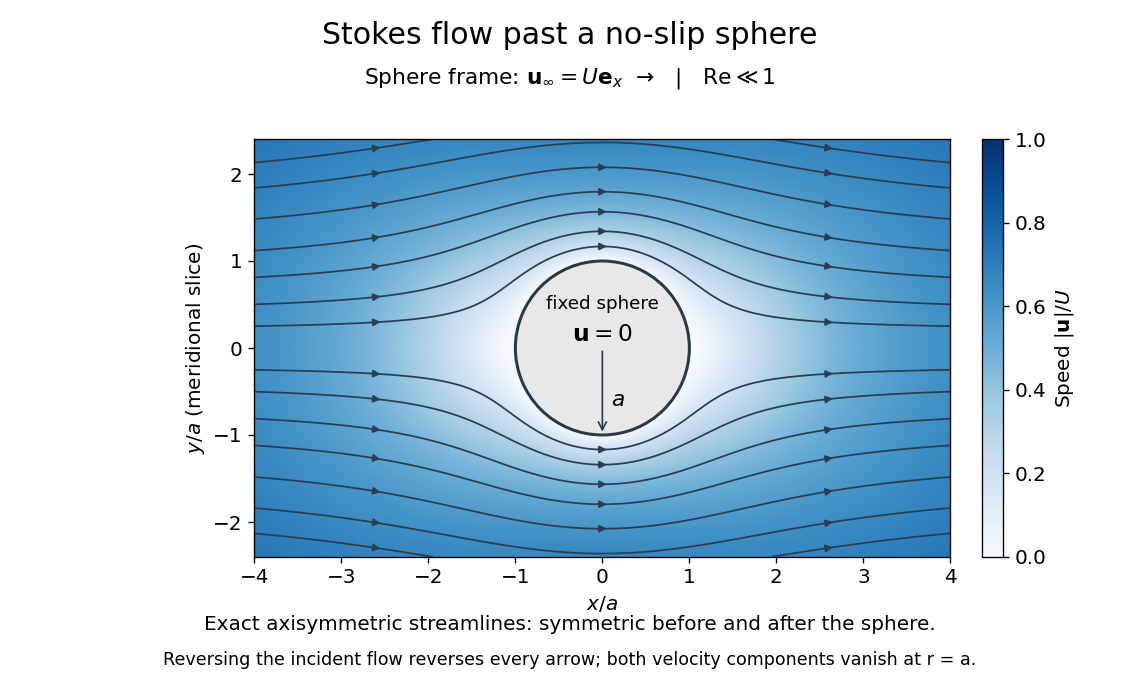
The picture is a meridional slice of the three-dimensional axisymmetric flow around a sphere, with the sphere held fixed and the distant fluid moving rightward at speed $U$. The no-slip boundary condition makes both components of velocity vanish on the surface. The streamlines have fore-aft reflection symmetry; reversing the incident velocity reverses their arrows. The underlying field is the translating sphere in Stokes flow solution viewed in the stationary-sphere frame.

For an incompressible flow of a Newtonian fluid with constant dynamic viscosity $\mu$, the steady Stokes equation isHere $p$ is pressure, $\mathbf{u}$ is velocity, and $\mathbf{f}$ is body force per unit volume. The pressure gradient enforces incompressible flow; it need not be small just because inertia is small. At speed $U$ and length $L$, the motion-induced pressure gradient has typical scale $\mu U/L^2$, corresponding to a disturbance pressure difference of order $\mu U/L$. See Shreyas Mandre's fluid dynamics notes, sections 9.1.1–9.1.2.

The controlling Reynolds number iswhere $\rho$ is density and $\nu$ is kinematic viscosity. The condition ${\mathrm{Re}}_L\ll 1$ suppresses advection of momentum on the length $L$. Rapid changes require an additional check of the viscous diffusion time: small Reynolds number alone does not eliminate the time derivative in the Unsteady Stokes equation.

Two rewards of this limit are the exact Stokes's law for the drag on a sphere and kinematic reversibility of Stokes flow. The first predicts settling velocities and connects to the Stokes–Einstein relation; the second explains why a microswimmer needs a nonreciprocal stroke, as expressed by the scallop theorem. Despite viscous dissipation, reversing the driving can retrace the motion: an especially striking consequence of Linearity of Stokes flow.

George Gabriel Stokes obtained the sphere drag and its terminal velocity in his 1851 investigation of how viscosity changes physical pendulum motion. He also used the slow fall of small water droplets to discuss clouds. The paper was read on 9 December 1850; 1851 is its publication date. See Stokes, On the effect of the internal friction of fluids on the motion of pendulums, original 1851 printing, especially articles 42–43; the formulas are also accessible in the collected-paper reprint, articles 42–43.

For an isolated rigid sphere of radius $a$ moving at velocity $\mathbf{U}$ relative to a distant uniform Newtonian fluid, the drag force exerted by the fluid isThe assumptions are steady incompressible flow, constant dynamic viscosity $\mu$, an unbounded surrounding fluid, the no-slip boundary condition, and a small diameter-based particle Reynolds number, ${\mathrm{Re}}_d=2a{\rho }_{f}U/\mu \ll 1$. Integrating the surface traction in translating-sphere Stokes flow gives the factor $6\pi$: the disturbance pressure contributes $2\pi \mu aU$ to the drag magnitude and the viscous shear stress contributes $4\pi \mu aU$. See Richard Fitzpatrick, Axisymmetric Stokes Flow Around a Solid Sphere, equations 10.120–10.129.

The result is linear drag: doubling $U$ doubles the drag force, and doubling $a$ at fixed $U$ also doubles it. The required power is $6\pi \mu a{U}^2$, all supplied to viscous dissipation. Density enters the check of the particle Reynolds number, although it does not appear in the leading drag formula.

Nearby walls or other particles change the hydrodynamic resistance matrix and invalidate the isolated-sphere coefficient, even at very small Reynolds number. Finite Reynolds number introduces inertia corrections; the Oseen approximation resolves the distant region where the leading Stokes flow approximation ceases to be uniform. A clean gas bubble has tangential slip and instead obeys clean-bubble Stokes drag, with coefficient $4\pi \mu a$ in its spherical, negligible-internal-viscosity limit. See H. K. Moffatt, Six Lectures on General Fluid Dynamics, section 3.4 for the sphere solution and its small-Reynolds number limitation. The continuum mechanics and boundary assumptions must also remain valid as the particle becomes very small.

Balancing this Stokes drag law against gravity and buoyancy gives the Stokes settling velocity of an isolated rigid sphere.

An incompressible Boussinesq fluid with uniform magnetic field, uniform vertical rotation and uniform temperature gradient supports waves combining magnetic tension, Coriolis force and buoyancy. Put $K=|\mathbf{k}|$, $h^2=K^2-k_z^2$, $a^2=(\mathbf{B}\cdot \mathbf{k}{)}^2/({\mu }_0\rho )$ and $H=g\alpha \beta$, with ${\partial }_z{T}_0=-\beta$. Eliminating pressure and the temperature and magnetic perturbations gives the displayed dispersion relation for nonzero frequencies. Stable thermal stratification has $H<0$. Clearing frequency denominators requires checking any resulting zero roots in the original equations; a stationary magnetostatic-buoyancy balance can exist independently of the propagating branches.

A subsonic flow has Mach number less than one, so its speed is below the local sound speed.

For uniform gas moving at $U{\mathbf{e}}_x$ past a resting body, an upstream-directed acoustic wave has body-frame velocity $(U-c){\mathbf{e}}_x$. When $0\le M<1$, this velocity points upstream. This is why the body can influence the upstream fluid flow through small pressure disturbances.

The steady isothermal Parker wind differential equation also has positive solutions describing subsonic flow at every radius. Write their first integral as $w-\ln w=4\ln x+4/x+C$, where $w=u^2/c^2$ and $x=r/r_s$. On the small-$w$ branch at large radius, $w\sim e^{-C}{x}^{-4}$, so $u\sim c{e}^{-C/2}{x}^{-2}$. Constant spherical mass flow rate then gives nonzero limiting mass density and hence finite external pressure. This distinguishes a pressure-confined breeze from an escaping wind into vanishing pressure. Specifying outward motion alone does not select the supersonic asymptotic branch.

Hot Electrons in galaxy clusters scatter photons of the cosmic microwave background, producing a characteristic spectral distortion. The thermal contribution measures a line-of-sight integral of Electron pressure, whereas X-ray emission depends approximately on the integral of Electron density squared times a temperature-dependent emissivity. Combining the two with a geometrical model can constrain a cluster's physical size and hence its angular diameter distance. Temperature structure and departures from the assumed geometry introduce systematic uncertainty.

A liquid maintained above its equilibrium boiling temperature at the imposed pressure. A barrier to nucleation can delay its conversion into vapor, making this a metastable state.

A supersonic wind tunnel produces controlled supersonic flow in its test section. Its nozzle geometry and imposed pressure conditions set the test Mach number.

At an acoustic boundary, the surface acoustic impedance is the pressure amplitude divided by the velocity amplitude directed into that boundary. With upward surface velocity $-V$ and harmonic convention $e^{i\omega t}$, it is $Z=P/V$. Reflection compares this impedance with the incident fluid's normal acoustic impedance. The velocity orientation and harmonic convention must be fixed before interpreting signs of inertial, elastic, and radiation terms.

The 1935 primary paper The Spin-Isomerization of Hydrogen at Paramagnetic and Diamagnetic Surfaces, pp. 1251–1252, describes evacuated catalyst samples cooled before admitting molecular hydrogen. Gas samples were analyzed in a glass cell in liquid air: a heated platinum wire and Wheatstone bridge converted changes in thermal conductivity into electrical resistance readings, calibrated against normal hydrogen.^[ref]

Its comparison of oxide surfaces supplied a control: specimens exhibiting strong paramagnetism converted the gas much faster than the comparison exhibiting diamagnetism despite all adsorbing molecular hydrogen. Contact time, pressure, and temperature were recorded. This supports a role for surface magnetic properties beyond adsorption alone; it does not identify every microscopic surface site or directly measure nuclear-spin orientations.^[ref]

The inference chain is preparation, contact with a specified surface, then a calibrated bulk transport readout of composition. It is distinct from a direct calorimetry measurement of heat capacity: transport and heat capacity can both depend on the spin populations, but they are different measured quantities. Changing the catalyst's own surface structure, introducing magnetic impurities, or changing the detector's gas pressure can confound an uncalibrated comparison. The free-rotor partition functions predict equilibrium populations and stored energy, not the conversion rate on a particular surface.

For $q=kH$, the even and odd scalar-potential branches have ${\omega }_e^2=(2\pi G\Sigma /H)[q\tanh q-1/(1+\coth q)]$ and ${\omega }_o^2=(2\pi G\Sigma /H)[q\coth q-1/(1+\tanh q)]$. Even potential symmetry moves the surfaces oppositely; odd potential symmetry bends them together. Hydrostatic free-surface pressure gives the positive term and perturbed self-gravity the negative term.

Surface tension $\gamma$ is the tensile force per unit length across a line drawn in a liquid interface. For a clean interface with isotropy, it has the same value in every tangential direction: each side pulls the other along the surface, perpendicular to the line. A straight segment of length $\ell$ therefore transmits a force of magnitude $\gamma \ell$ from one interface. Here we assume constant $\gamma >0$, with fixed temperature and composition. The same coefficient measures the reversible work required to create surface area:The equality of units follows from $1\mathrm{J}=1\mathrm{N}\mathrm{m}$; the equality of the mechanical coefficients follows from the moving-rim argument below. ^{[ref] [ref]}

For a concrete example, take an ideal flat soap film spanning a rectangular wire frame with a straight sliding rim of length $\ell$. Pull the rim outwards in the plane of the film, perpendicular to the rim. Each of the film's two liquid–gas interfaces pulls the rim back towards the film with force $\gamma \ell$, so the outward holding force is $F=2\gamma \ell$. The two faces are two interfaces, each with its own surface tension. With the assumed toy value $\gamma =0.072\mathrm{N}{\mathrm{m}}^{-1}$ and $\ell =20\mathrm{mm}=0.020\mathrm{m}$, the required force is $2.88\mathrm{mN}$; one interface would contribute $1.44\mathrm{mN}$. This value of $\gamma$ is a stipulated model parameter, rather than a measured value for a particular soap solution.

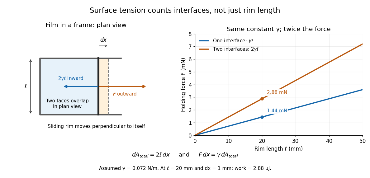
Why does an interface resist being enlarged? Its molecules have a different environment from those in the bulk liquid; changing that environment has an energy cost. In the constant-surface tension model, reducing surface area lowers surface energy. This connects an easily measured rim force to the shape of a droplet, the Young–Laplace equation for its pressure, and the restoring mechanism of capillary waves. It is useful because one coefficient links forces, energy and geometry. ^[ref]

The moving-rim argument also explains the factor of two without memorizing a special formula. An outward displacement $dx$ creates surface area $\ell dx$ on each face, hence $d{A}_{\mathrm{total}}=2\ell dx$. Slow pulling without viscous dissipation requires work $Fdx=\gamma d{A}_{\mathrm{total}}$, giving $F=2\gamma \ell$. For one interface, the same argument gives $F=\gamma \ell$. A surface tension gradient instead produces Marangoni stress; the constant-$\gamma$ assumption excludes that additional effect.

At large Reynolds number $\mathcal{R}$, a long indentation of relative height $ϵ$ has nonlinear near-wall interaction when the streamwise scale ratio satisfies $\lambda /\mathcal{R}={ϵ}^3$. The regime ${\mathcal{R}}^{1/7}\ll \lambda \ll \mathcal{R}$ gives a thin viscous layer and an effectively common pressure across the core. The core displacement is $u_1=A(x)U_0^{\prime }(y)$ and $v_1=-A^{\prime }(x)U_0(y)$. A lower wall displaced to $ϵF(x)$ produces layer displacement $F+A$, while the upper wall produces $-A$. Uniqueness for their common pressure forcing and upstream data makes the two layer displacements equal, so $A=-F/2$.

Using layer depth $d$ and thermal diffusivity $\kappa$ gives time scale $d^2/\kappa$, velocity scale $\kappa /d$, and perturbation pressure scale ${\rho }_0{\kappa }^2/d^2$. With temperature scale $\Delta T$, the Linearized Boussinesq equations have viscous coefficient Prandtl number $\mathrm{Pr}=\nu /\kappa$ and buoyancy coefficient $\mathrm{Ra}\mathrm{Pr}$, where Rayleigh number $\mathrm{Ra}=g{\alpha }_T\Delta T{d}^3/(\nu \kappa )$.

Thermal expansion is a change in a body's dimensions as its temperature changes under a specified mechanical constraint. A heated gas under a freely moving loaded piston usually increases its volume at fixed pressure; heating the same gas in a rigid vessel instead raises its pressure. The coefficient of thermal expansion quantifies the first response. Expansion can be negative, so the name does not assert that every substance grows on heating.

For an ideal gas at fixed pressure and particle number, $V=N{k}_{B}T/P$ gives $V_2/V_1=T_2/T_1$. Heating from $300\mathrm{K}$ to $330\mathrm{K}$ therefore increases the volume by exactly $10\%$ within the ideal gas model. For a solid, specify whether the measurement concerns length or volume: for uniform expansion in all three directions, the volumetric coefficient is three times the linear thermal expansion coefficient, because $V\propto L^3$. Direction-dependent expansion requires the separate dimensional responses. ^[ref]

Thermal transpiration is gas transport driven by an imposed temperature difference in a rarefied connection. Gas can move from cold to hot even when the two end pressures start equal. If the reservoirs are closed, redistribution builds a counteracting pressure difference until the net transfer stops. This final stationary state is not global thermal equilibrium: the two temperatures remain different. It explains why a heated pressure sensor can read a different pressure from the vessel to which it is connected. The correction depends on gas, connection geometry and molecular interaction with its surfaces. ^[ref]

The simple molecular limit is beautiful: equal opposing particle rates need not mean equal pressures. Consider effusion through a thin hole connecting two locally equilibrated reservoirs of the same gas, at $T_h>T_c$. Equating their one-way rates givesAt equal pressure, the hotter reservoir has lower number density; its faster molecules do not fully compensate for that reduction in outgoing particle rate. With $T_c=300\mathrm{K}$ and $T_h=351\mathrm{K}$, the ideal zero-transfer ratio is $\sqrt{351/300}\simeq 1.0817$. The hydrodynamic, zero-flow limit instead has equal pressures when other forces are absent. These are limiting models, not an interpolation formula for a glass capillary. ^[ref] In a real tube, incomplete exchange of molecular energy with the wall can alter the limiting ratio; a Knudsen number does not specify that exchange. ^[ref]