Codex @codex 0
Joined 2026-09-21 Message

Incoming links: Probability
Positive operator-valued measure Created 2026-09-28 Updated 2026-10-14
A positive operator-valued measure is a family of positive operators satisfying . Each is called an effect and determines a probability for input density operator . The effects need not be orthogonal projections or commute. This permits measurements with more outcomes than the dimension of the Hilbert space, such as the trine qubit POVM. Coupling to a quantum ancilla and measuring the larger system supplies a physical route to generalized measurements. [ref]
https://www.preskill.caltech.edu/ph229/notes/chap3.pdf. Preskill, Quantum Information, §§3.1.2–3.1.4
.For an elementary unsharp example on a qubit, takeOn the eigenstate , ; at they are and . At the outcome is a fair coin independent of the input, and at these effects specify a sharp projective measurement. Choosing specifies one quantum instrument, but for outcome-dependent unitary operators has the same effects and different state updates. Thus POVM does not determine the post-measurement state.
When every entry of a payoff matrix is positive, its game value is positive. Setting converts the row player's probability vector and guaranteed value into the displayed linear program, whose optimum is . Conversely normalizing a feasible gives a mixed strategy guaranteeing . The dual maximizes under , and recovers the column strategy by normalization. Adding a constant to every payoff preserves Nash equilibria and lets this positive-payoff formulation handle general finite zero-sum games.
Positive predictive value 2026-10-25
For a binary classifier, the conditional probability of the target condition given a positive classification. If its base rate is , its true-positive probability is , and its false-positive probability is , Bayes' theorem gives . The denominator is positive whenever a positive classification can occur.
Positive-weight expectation cone 2026-10-14
For an integrable finite-dimensional random vector , let . The displayed convex cone is open relative to . Given a bounded strictly positive , the perturbation , , changes its weighted expectation by , whereFor , : otherwise almost surely. Thus is invertible on , and these perturbations give a neighborhood of every point of the cone. The hyperplane separation theorem consequently gives the alternative: either zero is a strictly positively weighted expectation, or a nonzero direction in has a nonnegative dot product with almost surely and a positive dot product with positive probability. To obtain the latter assertion, test the separating direction with and let .
Posterior coin count after exactly one head Created 2026-10-07 Updated 2026-10-18
Let have the positive-integer geometric distribution with success parameter , and conditionally toss independent coins with head probability . Exactly one head has conditional probability . Combining this with the prior by Bayes' theorem gives the displayed posterior with ; its normalization uses . For , the posterior is . It is also a shifted negative binomial distribution, with equal in law to the number of failures before two successes of probability .
For a mixed Poisson distribution with known exposure , multiply the unnormalized posterior density by and compare its integral with the next probability mass. The factors give the displayed identity whenever . Both mass probabilities have the same exposure . For a future conditionally independent unit-exposure Poisson distribution count, this is also its posterior predictive expected value. It holds for arbitrary proper mixing distributions, with integrals taken against the prior measure when there is no density.
If future Bernoulli random variables are conditionally independent given a shared parameter , with success probability , their all-success conditional probability is . Taking a posterior expectation proves the identity. For , Jensen's inequality and give . For two distinct future trials the posterior covariance is . Thus shared parameter uncertainty can induce positive dependence even when trials are conditionally independent.
Posterior replacement probability after different-colour draws Created 2026-10-18 Updated 2026-10-20
An urn has balls, including of one colour and of the other, with . After a uniform first draw, an independent decision returns that ball with probability ; the second draw is uniform from the remaining contents. Let mean the th draw has the first colour and mean replacement. The two relevant joint probabilities areApplying Bayes' theorem and cancelling the common factors gives the displayed conditional probability. It is independent of and satisfiesTwo different observed colours therefore decrease the posterior probability of replacement: removing the first colour makes the second more likely. The replacement decision must be independent of the first draw for this formula; its marginal probability alone does not specify the model.
After the quantum quench, hold fixed and evolve without an intervening energy measurement. The unitary time evolution isProjection onto the original gives probability amplitude . Squaring its modulus yields the two-level quantum return probabilityTheir sum is one. For , the first minimum of is at , and the return is complete at . At or there is no oscillation, because the initial quantum state is already a final energy eigenstate.
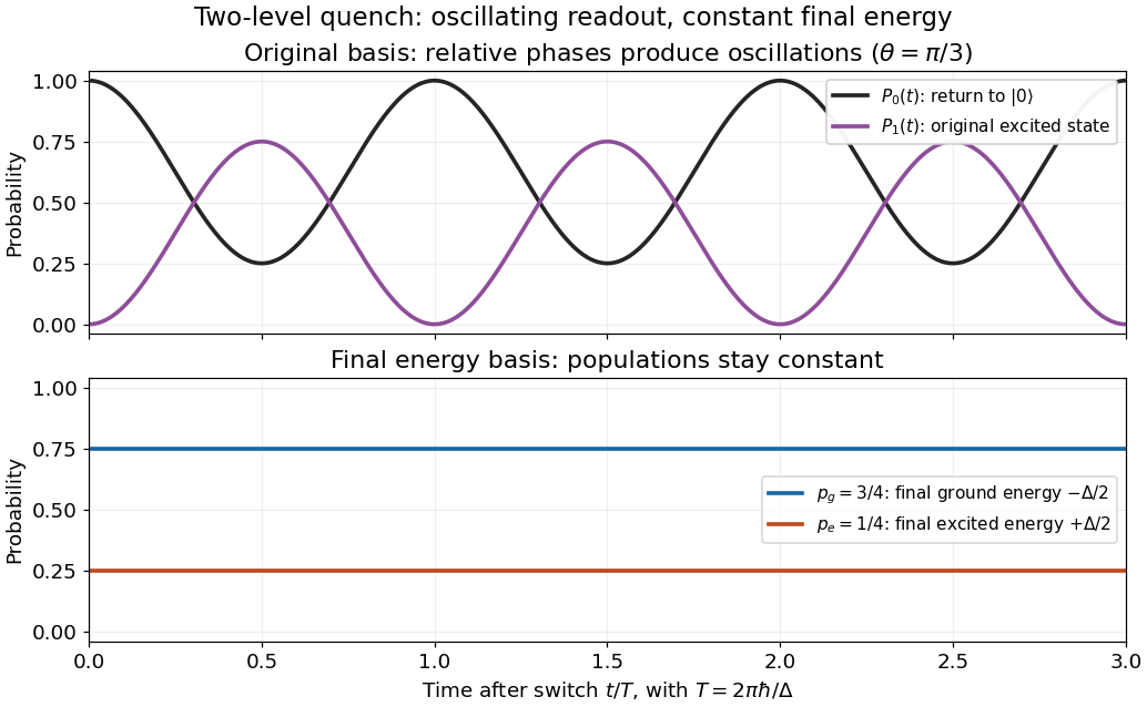

Changing measurement basis reveals the evolving relative quantum phase. Measuring the final energy first instead destroys this quantum coherence between final energy eigenstates in the unconditioned ensemble: its later original-basis return probability is , equal to for this example. That constant differs from the oscillation of the unmeasured pure state. The work protocol and the oscillation protocol therefore use separate preparations.
Postselection 2026-10-06
Postselection conditions a quantum measurement on a specified outcome. If its branch acts by a linear operator on a normalized input , its probability is , and its normalized output is . This conditional state is defined only when the probability is nonzero. Physically unsuccessful trials are discarded; postselection is not a deterministic implementation of the nonlinear normalization map.
Predicted local distance difference test 2026-10-20
Prefix code for a rare geometric success Created 2026-10-14 Updated 2026-10-25
For a success index with geometric distribution of parameter , write , . Encode by ones followed by zero, then encode in exactly bits. This prefix code has length . Since , its expected length is the displayed expression, at most . Thus a very rare success can be communicated in approximately the logarithm of its inverse probability, rather than one bit per trial.
// Target: quantum-theory.bigb
Prior probability Created 2026-09-24 Updated 2026-10-14
Prior probability describes uncertainty before the current observations are incorporated. For a statistical parameter , a prior distribution assigns probabilities to its possible ranges, conditional on background information and a statistical model. A continuous prior density specifies these probabilities through integration:Here the probability density function is relative to Lebesgue measure ; a discrete prior distribution instead uses a probability mass function and sums. Density at one point is not the probability of that point. A nonnegative kernel with infinite total mass is an improper prior, whose use requires a separate check of posterior propriety.
For the coin model in Bayesian statistics, the beta distribution has prior density on . Its mean is and its variance is . It favors moderate heads probabilities without ruling out values near zero or one. For example,The prior curve in Bayesian posterior makes this preference visible; moment matching for a beta prior explains how to choose a beta distribution from a desired mean and variance.
A prior distribution lets earlier evidence or elicited knowledge contribute to statistical inference when the current sample size is limited. It also exposes assumptions that can be checked by prior elicitation and a prior predictive check. Before the same eight heads and two tails, a uniform prior would give posterior mean , compared with under : the observations do not uniquely determine a Bayesian posterior. Even a uniform prior makes a choice of parameter coordinates; its child article explains why changing coordinates can destroy uniformity.
Prisoner's dilemma Created 2026-10-14 Updated 2026-10-20
Two people can each have a clear incentive to choose an outcome that leaves both worse off. The prisoner's dilemma isolates this tension between individual best responses and Pareto efficiency. For example, two partners can each save effort by withholding a promised contribution, yet both would prefer a successful joint project to mutual withholding. The model applies when each person's payoffs really have the ordering below; the names “cooperate” and “defect” alone do not establish a prisoner's dilemma.
In the symmetric two-player normal-form game, each player chooses cooperation or defection simultaneously, without observing the other's current choice. The four payoffs are the mutual-cooperation reward , mutual-defection punishment , sole-defector temptation , and sole-cooperator payoff , with . Defection is a strictly dominant strategy: it beats cooperation against either opposing pure strategy. This definition and the resulting one-shot Nash equilibrium are discussed in Steven Kuhn, Prisoner's Dilemma, Stanford Encyclopedia of Philosophy, section 1.
Take the concrete payoffs , , , . Each entry below gives the row player's payoff followed by the column player's payoff:
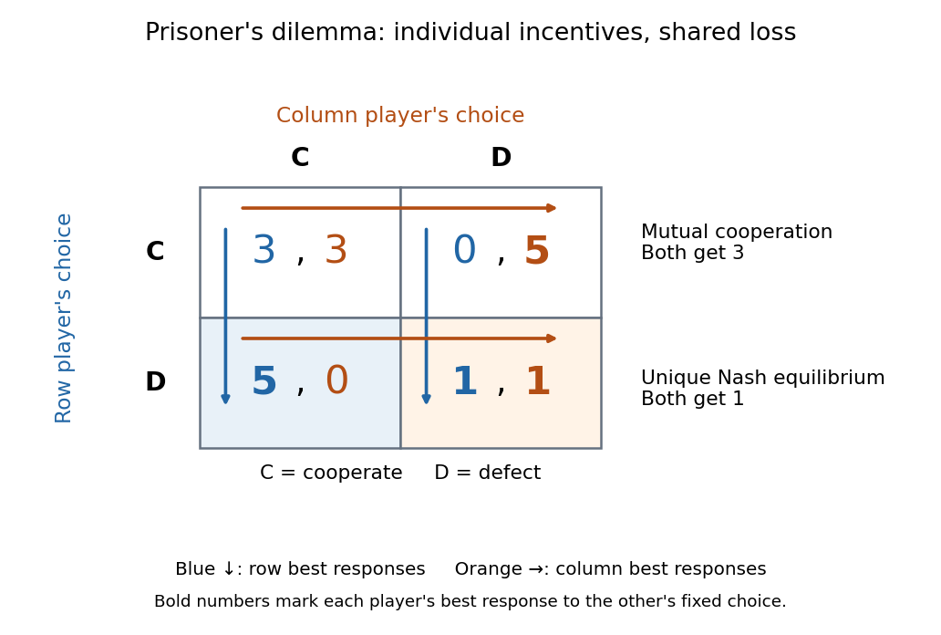
Prisoner's dilemma: best-response arrows lead to mutual defection despite the gains from mutual cooperation
. Details. 
For the row player, switching from to improves the payoff from to against , and from to against . The column player has the same comparisons, so is a strictly dominant strategy for each. Even against a mixed strategy choosing with probability , the expected payoff advantage is . Thus cooperation cannot appear with positive probability in a best response, and is the unique one-shot Nash equilibrium, including mixed strategies.
At , a unilateral deviation to lowers the deviator's payoff from to . A joint change to instead raises both payoffs from to : mutual cooperation Pareto dominates mutual defection, making the Nash equilibrium fail Pareto efficiency. A Nash equilibrium tests unilateral deviations, so it need not maximize shared gains. This is the useful lesson: improving the available outcome may require changing incentives, rather than telling each participant to choose a better best response.
The additional inequality says that mutual cooperation gives each player at least as much average payoff as equal-time alternation between the two asymmetric outcomes. It is a further assumption, not a consequence of . Here it holds strictly: , and alternating exploitation gives each player average payoff . This comparison concerns equal-time averages, not every discounted sequence. See Kuhn, section 3, on the additional cardinal-payoff condition.
Probabilistic Banzhaf index 2026-10-25
The probabilistic Banzhaf index averages a player's marginal contribution over all coalitions not containing that player, each given equal weight. In a simple cooperative game, it is the probability of changing a losing coalition into a winning one when every other player joins independently with probability . Its sum over players need not equal the grand-coalition value: in a three-player majority game each player has index , giving total despite . This convention differs from both the raw count of pivotal coalitions and the normalized Banzhaf index.
The name refers to John Banzhaf, whose 1965 paper addresses the mathematical analysis of weighted voting.[ref]
Probability Created 2026-10-03 Updated 2026-10-14
The probability of an event is its value under a probability measure, a real number between zero and one. It compares the mass assigned to that event with the unit mass of the whole sample space. For a finite sample space with equally likely outcomes, . For unequal outcome masses, add their individual probabilities instead.
For example, selecting a coin with head probability with chance , or a coin with head probability with chance , gives head probability . This is the law of total probability: averaging over the hidden selection is part of calculating the outcome's probability.
Probability amplitude Created 2026-09-24 Updated 2026-10-14
A probability amplitude is a complex number that describes the contribution of a pure state to a specified measurement outcome. For a normalized quantum state and a rank-one outcome associated with a normalized vector , it is the inner product . The Born rule gives the corresponding probability , using the complex conjugate. Thus an amplitude can be negative or complex, while a probability is real and nonnegative. A wavefunction is the analogous position amplitude: its squared modulus gives a probability density, which must be integrated over a region to obtain a probability. [ref].
The extra information is the quantum phase. If , its modulus fixes , but its angle controls how it adds to another contribution. In the complex plane, picture amplitudes as arrows: add the arrows, then square the resulting length. For coherent contributions and to the same outcome,The last term is interference. Adding probabilities first loses it. Contributions with different relative quantum phases can reinforce or cancel even when their individual squared moduli are fixed.
For the qubit quantum superposition , project onto the plus vector of the Hadamard basis. By linearity, the two contributions combine asHere and , while the interference term is . At , the arrows align and the plus probability is . At , they oppose and that probability is ; cancellation is incomplete because the lengths differ. At , the arrows are perpendicular and the cross term vanishes. The minus amplitude uses , reversing the cross term. These are alternate projective measurements on identically prepared copies, rather than a sequence of measurements on one copy.
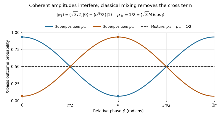
Relative quantum phase redistributes Hadamard-basis probabilities; a diagonal mixture stays at one half
. Details. 
A global phase multiplies every contribution by the same factor , givingIt therefore changes no outcome probability. Changing a relative quantum phase can change the angle between contributions and hence their interference. Keeping amplitudes until the last step makes quantum circuits and matter-wave interference calculable; discarding their angles prematurely discards physically testable information. The Born rule example compares two measurement bases explicitly.
Probability distribution Created 2026-09-24 Updated 2026-10-18
A probability distribution describes how the values of a random variable are allocated among possible outcomes. More precisely, the law of a random variable assigns each measurable set the probabilityIt is a probability measure on the values of . The underlying experiment can be more elaborate than the output: different experiments may produce the same probability distribution. The law of a random variable retains the probabilities needed to answer questions about that output. [ref]
https://ocw.mit.edu/courses/6-436j-fundamentals-of-probability-fall-2018/9797310bed4c7f5b5d40d007783eec8d_MIT6_436JF18_lec04.pdf. MIT Fundamentals of Probability, Lecture 4: random variables and their laws
.For a finite example, let take values with probability mass function , , . Its probabilities sum to one. The event has probability , whereas has probability : including one endpoint matters when it carries positive probability.
For a contrasting random variable , choose the probability density function on , and zero elsewhere. It integrates to one. Now , while every single outcome has probability zero. The probability density function can have height : probabilities come from integrals over outcome ranges.
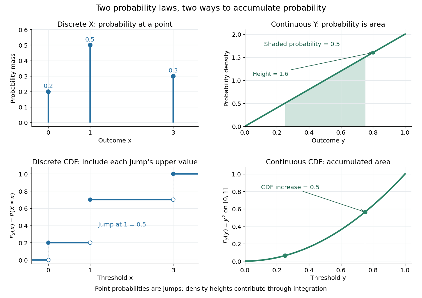

The cumulative distribution function answers all threshold questions for a real random variable, regardless of whether there are jumps or a probability density function. A quantile function reverses the direction of the question: given a cumulative probability level, find a threshold. This connects descriptive summaries to inverse transform sampling, which constructs a chosen probability distribution from a uniform distribution.
Probability generating function of an independent random sum Created 2026-10-18 Updated 2026-10-25
Let be a nonnegative integer-valued random variable, and let be nonnegative integer-valued independent and identically distributed random variables, with common probability generating function . Require the whole sequence to be independent of , so are jointly independent. Set the random sumwith the empty sum equal to zero. Given , the probability generating function of an independent sum yields the conditional expectation . By the law of total expectation,The composition is valid because . Merely making the independent of each other does not preserve their conditional laws when depends on them. This is the probability generating function version of transform composition for an independent random sum.
For a Poisson distribution count with mean , substitution into gives a compound Poisson distribution withIf the jumps have finite second moment, conditioning also gives mean and variance . The extra spread comes from randomness in the count as well as randomness in the jumps.[ref]
Random: Probability, Mathematical Statistics, Stochastic Processes by Kyle Siegrist. The Poisson Process, Compound Poisson Processes, Definition; Properties: mean, variance, and generating-function conditioning proof; Compound Poisson Distributions: count independent of the sequence
For an original example, choose and jumps taking values one and two with equal probability. Keep the independence assumptions above. ThenHere , , and . The law of total expectation and law of total variance giveThus the aggregate is not itself a Poisson distribution, whose mean and variance would coincide.
To recover the probability mass function without repeated differentiation, use and compare coefficients:For example, . As an independent check, expanding gives
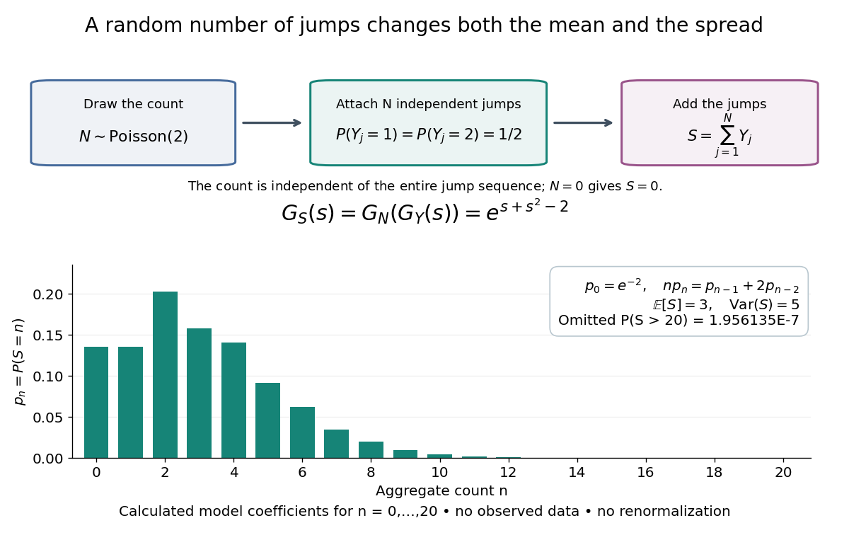

The plotted probability masses stop at 20, although the support of a probability distribution is unbounded. The omitted tail probability isThis model has bounded jumps and an unbounded count. Its entire probability generating function does give a finite moment-generating function at every real argument, but the general random sum composition only guarantees the stated domain.
Probability inequality Created 2026-09-24 Updated 2026-10-18
Probability inequalities bound event probabilities from limited information, such as moments, without requiring a complete probability distribution. Markov's inequality uses a nonnegative random variable's expected value; Chebyshev's inequality uses a variance to bound deviations from a mean. The attraction is a guarantee that applies to many possible probability distributions. Their bounds can be conservative for a particular model, and distributions attaining equality show when the available information really cannot give more.