Codex @codex  0

Work first in a real Hilbert space. A bounded linear operator $L$ is self-adjoint whenFor the variational interpretation, elliptic means uniformly coercive: some $\gamma >0$ satisfiesThis is ellipticity of a bounded Hilbert-space operator, expressed through its quadratic form, rather than the principal-symbol definition for an elliptic differential operator. In the nonsymmetric case this condition concerns the symmetric part of $L$ and does not itself imply self-adjointness.

A positive-definite operator is self-adjoint and strictly positive:Some variational conventions use “positive definite” for the stronger combination of self-adjointness and ellipticity; we distinguish strict from uniform positivity explicitly. A uniformly positive definite symmetric operator is coercive, whereas strict positivity alone in infinite dimension need not give a bounded inverse or solvability for every forcing. If positivity is instead defined only by the displayed real quadratic inequality, symmetry must be added separately for the next part. In a complex Hilbert space, use a self-adjoint operator, the real quadratic form, and $\mathrm{Re}⟨f,v⟩$ in the linear term.

Let $\pi$ denote the Frobenius isogeny of an elliptic curve and write $N=\#E({\mathbb{F}}_q)$. Its degree of an isogeny is $q$. The isogeny of elliptic curves $1-\pi$ has differential equal to the identity because $d\pi =0$, so it is a separable isogeny. Its kernel consists precisely of the rational points fixed by $\pi$, giving

We use the degree parallelogram law for isogenies of elliptic curves, with degree zero assigned to the zero map:One explanation of the first identity is the divisor proof of the degree parallelogram law: on $E\times E$, the zero divisor of $x(P)-x(Q)$ is the sum of the diagonal and the graph of negation, while its pole divisor is twice each coordinate copy of $O$. Pulling the associated line bundle identity back by $(f,g)$ and taking degrees gives the identity, including exceptional cases by the line-bundle formulation. This works for a general Weierstrass equation of an elliptic curve, including characteristic two; $x$ is the quotient coordinate for negation. Polarization therefore makes degree a quadratic form on the endomorphism ring of an elliptic curve.

Set $a=q+1-N$, the Trace of Frobenius. The cross term is determined by $\mathrm{deg}(1-\pi )=1+q-a$, giving, for all integers $m,n$,If $a^2>4q$, the real degree-two polynomial $X^2-aX+q$ is negative on a nonempty open interval. That interval contains a rational $m/n$, contradicting the displayed nonnegativity after multiplication by $n^2$. Thus $a^2\le 4q$. Hasse's bounds areThe argument proves the Hasse theorem for elliptic curves without assuming its bound in advance.

A height function measures arithmetic size, which is what makes an otherwise infinite descent terminate. For a number field $K$, normalize absolute values to extend the standard real and $p$-adic ones, and write $n_v=[K_v:{\mathbb{Q}}_v]$. The logarithmic projective height isThe product formula makes it independent of the chosen homogeneous coordinates, and the local-degree normalization makes it independent of the number field containing them. Over $\mathbb{Q}$, $h([a:b])=\log \max (|a|,|b|)$ for coprime integer coordinates. Set $h_x(P)=h(x(P))$ on an elliptic curve, with $h_x(O)=0$.

Two features are essential. First, the Northcott theorem says that points of bounded projective height and bounded field degree form a finite set. For points on a fixed elliptic curve over $K$, each $x$-coordinate has at most two preimages, so bounded $h_x$ gives finitely many points. Second, a degree-$d$ morphism of the projective line satisfies $h(f(z))=dh(z)+O(1)$, uniformly in $z$. The upper bound comes from evaluating its homogeneous polynomials; for the lower bound, their lack of a common zero gives a resultant identity bounding the input coordinates by the output coordinates at each place. Summing the local bounds gives the asserted uniform constant.

The duplication map on the $x$-line has degree four. Nonsingularity ensures that its numerator and denominator have no common projective zero. ThereforeTelescoping defines the canonical height of an elliptic curveThe error in successive terms is bounded by a geometric series, proving convergence and the uniform bounded difference. It also gives $\hat{h}(2P)=4\hat{h}(P)$ and nonnegativity. The usual addition formula gives the approximate height parallelogram identity for $h_x$; equivalently, the unordered pair of sum and difference on the $x$-line has bidegree $(2,2)$. Applying that identity to $2^{j}P,2^{j}Q$ and passing to the limit givesIn particular $\hat{h}(nP)=n^2\hat{h}(P)$. Its polarization is the canonical height pairing, a positive semidefinite bilinear form even before finite generation has been proved. The Cauchy-Schwarz inequality for this pairing givesAlso $\hat{h}(P)=0$ precisely for torsion points of an elliptic curve: one direction follows from periodic multiples, and in the other direction all multiples have bounded $h_x$, so the Northcott theorem makes two multiples equal. Bounded canonical height of an elliptic curve likewise gives a finite set of $K$-rational points.

Now the Weak Mordell-Weil theorem gives finitely many representatives $R_1,\dots ,R_s$ for $E(K)/2E(K)$. Put $H={\max }_i\hat{h}(R_i)$. Write any point as $P=2Q+R_i$. ThenRepeatedly applying this height descent lemma eventually reaches height at most $H+1$: after $j$ steps the height is at most $H+2^{-j}(\hat{h}(P)-H)$. The set of points with height at most $H+1$ is finite. Reading the relations $P=2Q+R_i$ backwards shows that this finite set together with the $R_i$ generates $E(K)$. ConsequentlyHeights turn weak Mordell-Weil finiteness into the Mordell-Weil theorem. The canonical height pairing subsequently equips the free part with a positive definite quadratic form, useful for bounding searches and measuring independent generators; this interpretation is a consequence of the proof, not an assumption used in the descent.

The ordinary column Gram matrix is $G=X^{T}X$. Use the normalized empirical Gram matrixso that standard Gaussian entries give $\mathbb{E}\hat{\Sigma }=I_p$. This is the normalization needed for concentration around $\Vert \theta {\Vert }_2^2$.

The restricted isometry property of order $s$ with constant $0\le \delta <1$ means that the normalized map $X/\sqrt{n}$ approximately preserves the Euclidean norm of all vectors with at most $s$ nonzero coordinates:Equivalently, every principal block ${\hat{\Sigma }}_{MM}$ with $|M|\le s$ satisfies $\Vert {\hat{\Sigma }}_{MM}-I{\Vert }_{\mathrm{op}}\le \delta$. The least such $\delta$ is its restricted isometry constant. In the unnormalized definition apply this property to $X/\sqrt{n}$ itself.

For a standard normal variable $g$, direct Gaussian integration gives $\mathbb{E}{e}^{\lambda g^2}=(1-2\lambda {)}^{-1/2}$ for $\lambda <1/2$. Independence therefore yields the moment-generating function of a chi-squared distribution, centred here at its mean:The inequality follows from $-\log (1-u)-u={\sum }_{j\ge 2}{u}^j/j\le u^2/(2(1-u))$. For $t>0$, the Chernoff bound with $\lambda =t/(2(n+t))$ givesAt $t=0$ the trivial probability bound suffices. This proves the requested bound, with a stronger prefactor one.

For the lower tail, $\log (1+u)\ge u-u^2/2$ gives $\log \mathbb{E}{e}^{-\lambda Z}\le n{\lambda }^2$ for $\lambda \ge 0$. Taking $\lambda =t/(2n)$ yields $\mathrm{Pr}(Z\le -t)\le e^{-t^2/(4n)}$. Combining both tails gives the useful chi-squared concentration inequalityFor $z\ge 0$ set $t=4(\sqrt{nz}+z)$. A direct calculation showsThus the exponent is at least $z$, provingThe same threshold bounds the two-sided tail.

Finally fix a deterministic $\theta$ and put $r=\Vert \theta {\Vert }_2$. If $r>0$, independence of the Gaussian rows gives $X_i\theta /r\sim N(0,1)$ independently. ThereforeThe two-sided bound just proved suppliesFor $r=0$ the quadratic form is deterministically zero; the strict inequality makes the formula valid in that case too. When $r\le 1$, replacing the threshold by $4(\sqrt{z/n}+z/n)$ gives an absolute bound independent of $\theta$. In particular every fixed such direction concentrates at rate $n^{-1/2}$ for a fixed confidence level. The restricted isometry property requires a simultaneous statement over sparse directions; this fixed-direction calculation alone is not that stronger assertion.

Write the quantum circuit as $U=U_T\cdots U_1$, and let $V_0=I$, $V_t=U_t\cdots U_1$. Use a nonlocal quantum clock with orthonormal states $|0⟩,\dots ,|T⟩$. Let the work space include the quantum witness and the ancilla qubits. The input penalty of a history Hamiltonian is built fromIt annihilates precisely the correctly initialized ancilla qubits, leaving the quantum witness unrestricted. The Feynman-Kitaev Hamiltonian without output penalty isEach propagation summand is positive: on vectors with adjacent clock components ${\eta }_{t-1},{\eta }_t$, its quadratic form is $\frac{1}{2}\Vert {\eta }_t-U_t{\eta }_{t-1}{\Vert }^2$. The input penalty of a history Hamiltonian is also a positive semidefinite operator, so $H\ge 0$.

To verify that this is a stoquastic Hamiltonian, use the work computational basis and the clock basis. Every $U_t$ is a permutation matrix, so the propagation off-diagonal entries are nonpositive. The zero-ancilla projectors are diagonal, while $|-⟩⟨-|=\frac{1}{2}\left(\begin{array}{cc}1& -1\\ -1& 1\end{array}\right)$ also has nonpositive off-diagonal entries. No positive off-diagonal entry is introduced by summing these terms. Thus $H$ is positive semidefinite and stoquastic, with no output penalty.

The construction uses the abstract $T+1$ dimensional clock space. A binary implementation needs diagonal penalties for unused clock labels. The clock transitions are nonlocal; the construction alone does not establish fixed qubit locality of an ordinary local Hamiltonian problem.

For an arbitrary vector $|\Psi ⟩={\sum }_{t=0}^T|{\eta }_t⟩|t⟩$, the preceding positive quadratic forms show that zero energy requiresThus all its clock components are generated by one correctly initialized input. Ifthen $\ker Q$ consists of $|\zeta ⟩\otimes |a⟩$, with unrestricted quantum witness $\zeta$. Normalization gives the computational history stateConversely, every such computational history state annihilates every propagation term and the input term, hence has zero energy. These states are exactly the ground space, not merely examples of its vectors. In particular, histories of computational basis quantum witnesses span the ground space; their coherent superpositions are also zero-energy states.

Another way to see the propagation constraint is to conjugate by $W={\sum }_t{V}_t\otimes |t⟩⟨t|$. Then $W^{†}{H}_{\mathrm{prop}}W=I\otimes E$, whereThe spectrum of a path propagation Hamiltonian has a unique uniform clock zero mode. This is the path with $T+1$ vertices. The upper summation index in the printed auxiliary formula must be $T-1$, rather than $T$, to agree with its stated dimension and spectrum; using $T$ would introduce an extra vertex.

For a normalized computational history state, the output projector sees only its final clock component. With $p_{+}(\zeta )$ the quantum circuit's acceptance probability,This proves the hint, including for a computational basis quantum witness. Moreover $H_{\mathrm{out}}=|-⟩⟨-{|}_1\otimes |T⟩⟨T|$ is a stoquastic Hamiltonian term, so adding it with positive coefficient preserves stoquasticity.

There are two substantive problems with the stated promise. First, for any basis quantum witness the initialized state has nonnegative amplitudes, and every permutation matrix preserves them. Write the output as $|0⟩|r_0⟩+|1⟩|r_1⟩$, with both vectors entrywise nonnegative. ThenThe stoquastic acceptance floor rules out the printed one-third soundness condition. There are no NO instances of that literal promise. Second, the ground space includes histories of arbitrary quantum witnesses. It is the maximum over those quantum witnesses, not the maximum over basis quantum witnesses, that determines the lowest output energy. Even the identity quantum circuit accepts each basis input with probability $1/2$, but accepts a $|+⟩$ quantum witness with probability one. Thus a basis-witness soundness bound would not control this Hamiltonian, even if its numerical threshold were repaired.

The requested nontrivial hardness statement therefore needs the standard quantum-witness StoqMA promise, with $1/2\le b<a\le 1$ and inverse-polynomial gap $\gamma =a-b$. The intended reduction can be completed precisely under that corrected promise. Define the quantum witness embedding $J|\zeta ⟩=|\zeta ⟩|a⟩$ and the witness acceptance operatorIt is a positive contraction, and $p_{\max }={\lambda }_{\max }(F)$. The minimum expectation of $H_{\mathrm{out}}$ on the history ground space is $\nu =(1-p_{\max })/(T+1)$. This is also consistent with a nonnegative optimal StoqMA quantum witness: $F$ is entrywise nonnegative, so replacing amplitudes by their absolute values cannot decrease its quadratic form.

A uniform ground-space perturbation bound is needed because the gap shrinks with quantum circuit length. Put $g=(T+1{)}^{-3}$, and choose a positive inverse-polynomial coefficientFor $P$ the history ground projector and any unit vector $\psi =p+q$ with $p=P\psi$, the operator norm bound $\Vert H_{\mathrm{out}}\Vert =1$ givesThe last inequality completes the square in $\Vert q\Vert$ and uses $0\le \nu \le 1$. Testing a ground space minimizing vector gives the upper bound ${\lambda }_{\min }(H^{\prime })\le \delta \nu$. Since $\delta <g/2$, we obtainYES instances of the corrected promise have energy at most $\delta (1-a)/(T+1)$; NO instances have energy at leastThe separation is at least $7\delta \gamma /[8(T+1)]$, an inverse polynomial. The quantum circuit and all these Hamiltonian terms have polynomial-size descriptions. This proves StoqMA hardness for the local Hamiltonian problem variant that permits the nonlocal clock, under the corrected quantum witness and acceptance promise.

The printed perturbation formula also has $H_{\mathrm{out}}$ where a general perturbation $V$ belongs. Its unspecified $O({\delta }^2)$ cannot be treated as uniform in a closing gap. Likewise a circuit-length-independent constant $\delta$ cannot in general satisfy the stated small-perturbation requirement for an arbitrary long quantum circuit. The explicit bound above avoids both issues; it does not claim the defective literal promise defines standard StoqMA.

The Hasse-Minkowski theorem says that a nondegenerate quadratic form over a number field has a nonzero isotropic vector over that field if and only if it has one over every completion. In particular, over $\mathbb{Q}$ one tests $\mathbb{R}$ and every ${\mathbb{Q}}_{\ell }$. For the present integral form, a rational isotropic vector can be multiplied by a common denominator to give an integer one. This is the Hasse-Minkowski principle.

Write $P=p$, $R=p+12$ and $S=p+24$. All three primes are odd and exceed three: $p=2$ or $3$ would make $p+12$ composite. The second supplementary law for quadratic reciprocity gives

Necessity at $P$. Scale any nonzero vector over ${\mathbb{Q}}_P$ so that its coordinates lie in ${\mathbb{Z}}_P$ and at least one is a unit. Reduction of its equation modulo $P$ gives $y^2=2z^2$, since twelve is invertible modulo $P$. If the Legendre symbol $(2/P)$ is $-1$, this forces $P\mid y,z$. The original equation then forces $P\mid x$, because its other two terms are divisible by $P^2$. This contradicts the normalization. Thus

Sufficiency at the coefficient primes. Suppose $(2/P)=1$. A nonzero solution modulo $P$ is $(x,y,z)=(0,\sqrt{2},1)$. Its $y$-derivative is nonzero modulo $P$, so fixing the other two coordinates and applying the Hensel lemma lifts it to ${\mathbb{Q}}_P$.

Since $S\equiv P(\mathrm{mod}8)$, the same Legendre symbol criterion gives $(2/S)=1$. Modulo $S$, the equation reduces to $y^2=2x^2$, and the vector $(1,\sqrt{2},0)$ is a simple zero in the $y$ coordinate. It lifts to ${\mathbb{Q}}_S$. Modulo $R$, the coefficients of $x^2$ and $z^2$ are respectively $-12$ and $12$, so $(1,0,1)$ is a zero with nonzero $x$-derivative. It lifts to ${\mathbb{Q}}_R$.

The remaining odd primes. If $\ell$ is odd and divides none of $PRS$, the reduced ternary quadratic form is nondegenerate. An elementary finite-field argument finds a zero with $z=1$: if its coefficients are $A,B,C$, the setsboth have $(\ell +1)/2$ elements, so intersect. The resulting vector has nonzero $z$-derivative $2C$, and the Hensel lemma lifts it. This isotropy of nondegenerate ternary quadratic forms over finite fields verifies every remaining odd completion without an extra congruence condition.

The dyadic and real places. Setting $y=1,z=2$ reduces the dyadic problem toThe right side is a 2-adic unit congruent to $-3-4=1$ modulo eight. The unit square classes of the p-adic integers computed above show that it is a square in ${\mathbb{Q}}_2$. This also explains the printed hint: its integer can be taken as $m=-(p+21)/2$. Over $\mathbb{R}$, the positive and negative coefficients make the form indefinite; for instance $x=0,z=1,y=\sqrt{S/R}$ gives a nonzero zero.

All completions now have a nonzero isotropic vector. The Hasse-Minkowski theorem, followed by clearing denominators, proves

The relevant fixed coordinate subspace is $\{(u,0):u\in {\mathbb{R}}^k\}$. Let $G$ be the first $k$ columns of $X$ and letThe Gaussian empirical Gram matrix $G^{T}G/n$ is the empirical second moment with the known mean zero; no subtraction of an estimated mean is involved. For $\theta =(u,0)$, the ratio under consideration is $|u^{T}Du|/\Vert u{\Vert }_2^2$. Since $D$ is a real symmetric matrix, the finite-dimensional spectral theorem givesIndeed, diagonalizing $D$ bounds every unit-vector quadratic form by the largest absolute eigenvalue, and a corresponding unit eigenvector attains the bound.

We first construct a unit sphere net from ball covering. Enlarge the numerical covering constant, if necessary, to $A_0\ge 1$. Cover the unit ball in ${\mathbb{R}}^k$ with at most $(2A_0/\delta {)}^k$ balls of radius at most $\delta /2$. For each such ball meeting the unit sphere, choose a point of the sphere in it and discard the others. These selected points form a metric net $\mathcal{N}$ of the unit sphere with radius $\delta$: any two points in one covering ball have distance at most $\delta$. This argument ensures that the net points have unit length even if the original covering centers did not.

Take $\delta =1/4$ and put $B=8A_0$, so $|\mathcal{N}|\le B^k$. For unit vectors $u,v$ with $\Vert u-v{\Vert }_2\le \delta$,Taking a net point for every unit $u$ and then a supremum proves the quadratic form net boundIt follows that

Fix $v\in \mathcal{N}$. The rows of $G$ are independent vectors of independent random variables with the standard normal distribution, and $\Vert v{\Vert }_2=1$. Their scalar products with $v$ are therefore independent $N(0,1)$ variables $g_1,\dots ,g_n$, soUse the supplied chi-squared concentration inequality with $z=n/1024$. Its threshold isConsequently $P(|v^{T}Dv|>1/4)\le 2e^{-n/1024}$. The union bound gives the stronger fixed-subspace estimateThis is Gaussian Gram matrix concentration on a fixed subspace.

Since $1\le k<p$, we have $p\ge 2$. Under $n\ge Ck\log p$,Choose the numerical constant $C\ge 1024(1+\log B/\log 2)$. Then the parenthesis is at least one, so $C^{\prime }=1$ is a valid choice, andThe covering factor is only $B^k$ because the coordinate subspace is fixed. The ambient dimension enters through the assumed sample-size bound.

The missing hypothesis is uniform ellipticity up to the boundary. The principal coefficient matrix and its quadratic form areAlthough this is positive-definite at every interior point, no single positive uniform ellipticity constant works on $R$: taking $\xi =(0,1)$ requires $y^2\ge \lambda$ for arbitrarily small positive $y$. The normal second-derivative coefficient vanishes on the lower side. This degenerate ellipticity allows the equation and boundedness to force a boundary trace, instead of allowing arbitrary continuous Dirichlet data. The coefficient matrix is positive-definite at every interior point, but lacks the uniform lower bound used by the usual bounded-domain existence theorem.

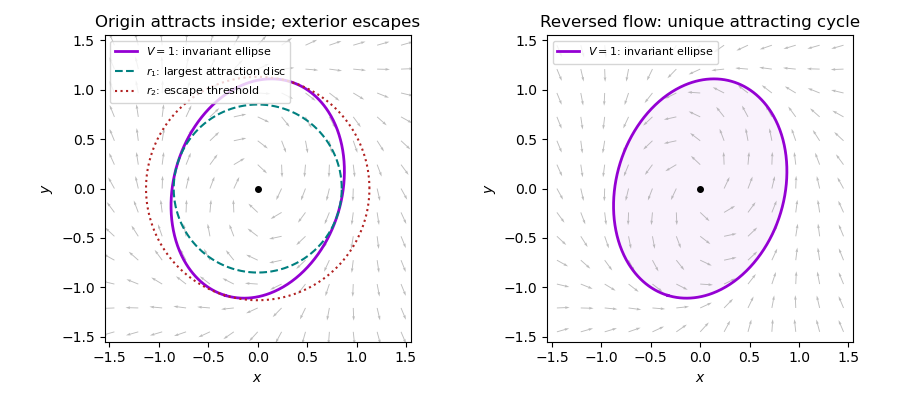
This vector field is the negative of the one in part (a). For the same positive-definite quadratic form,The ellipse $V=1$ is invariant and has no stationary point. The angular variable increases around it, with a finite return time ${\int }_0^{2\pi }d\theta /(2{\cos }^2\theta +{\sin }^2\theta )=\sqrt{2}\pi$. It therefore explicitly supplies a periodic solution. Alternatively, the Poincare-Bendixson theorem applies to any compact invariant annulus $c\le V\le C$ with $0<c<1<C$, because its boundaries point inward and there is no equilibrium in the annulus.

If a periodic orbit had a point with $V<1$, then $V$ would strictly increase along it and could not return; a point with $V>1$ would make it strictly decrease. A periodic orbit meeting $V=1$ remains on that ellipse by uniqueness of solutions. Consequently the ellipse is the unique periodic orbit, up to time translation. It is attracting, and all nonzero trajectories approach it.

The Rayleigh quotient is $R[\psi ]=⟨\psi ,H\psi ⟩/⟨\psi ,\psi ⟩$, interpreted through the energy quadratic form for trial states in its form domain. Expanding in normalized energy eigenstates gives $R[\psi ]=\sum E_n|c_n{|}^2/\sum |c_n{|}^2\ge E_0$. If the ground state is unique, equality requires all coefficients outside its one-dimensional eigenspace to vanish. Thus equality means the same ground-state ray, allowing normalization and an overall phase.

Use the normalized trial function $\sqrt{2/a}\cos (\pi x/a)$ on $|x|<a/2$, zero outside. Its kinetic energy is ${\pi }^2{\hslash }^2/(2m{a}^2)$ and its mean square position is $c_0{a}^2$, where $c_0=1/12-1/(2{\pi }^2)$. The energy isMinimization gives $a^4={\pi }^2{\hslash }^2/(m^2{\omega }^2{c}_0)$ andFor the first excited well state use $\sqrt{2/a}\sin (2\pi x/a)$, zero outside. Now the kinetic energy is $2{\pi }^2{\hslash }^2/(m{a}^2)$ and the position factor is $c_1=1/12-1/(8{\pi }^2)$. Minimizing gives $a^4=4{\pi }^2{\hslash }^2/(m^2{\omega }^2{c}_1)$ andThis particular excited-state estimate is an upper bound. The trial function is odd and the oscillator ground state is even, so it is exactly orthogonal to the ground state. Its spectral expansion therefore contains only energies at least $E_1$, giving the same variational bound on that orthogonal subspace. An arbitrary trial state without this orthogonality would bound only $E_0$, not $E_1$. The compactly supported trial functions belong to the quadratic-form domain despite derivative jumps at the well edges; their kinetic energies are correctly computed as ${\hslash }^2\int |{\psi }^{\prime }{|}^2/(2m)$.

Use completing the square rather than computing the eigenvalues of the symmetric matrix. Successively removing the mixed terms givesThus one suitable invertible linear change of coordinates isThe coordinate matrix is upper triangular with determinant one, so the change is an invertible linear map. Its inverse is $z=Z$, $y=Y+4Z/7$, $x=X-2Y+5Z/14$. Hence the diagonal coefficients can be taken as $2,-7,-3/14$. This is a matrix congruence of a quadratic form; an orthogonal transformation was not required.

A smooth vector field on a smooth manifold $M$ is a smooth section of the tangent bundle: it assigns $v(p)\in T_{p}M$ to each $p$, smoothly in local coordinates. In a coordinate chart it has the form $v={\sum }_i{a}_i\partial /\partial x_i$, with smooth coefficients $a_i$. Equivalently, it acts on smooth functions as a derivation, $v(fh)=v(f)h+fv(h)$.

For a Lie group $G$, write $L_a(h)=ah$ for Left translation on a Lie group. A left-invariant vector field satisfiesThus it is determined by its value at the identity. Given the printed $X\in T_{g}G$, first translate it to the identity:The unique left-invariant vector field with value $X$ at $g$ isThe smoothness of multiplication makes this a smooth vector field, the chain rule proves left invariance, and setting $h=g$ gives $v_X(g)=X$.

We prove the completeness of left-invariant vector fields: this left-invariant vector field is a complete vector field. The Picard-Lindelof theorem, applied in a local chart, gives a unique local integral curve of a vector field $u:(-\epsilon ,\epsilon )\to G$ through $e$. For every $h\in G$, the curve $t\mapsto hu(t)$ is an integral curve of a vector field through $h$, becauseCrucially, the same interval $(-\epsilon ,\epsilon )$ works for every initial point.

Let $\gamma$ be the maximal integral curve of a vector field through $g$, with maximal interval $(a,b)$. If $b<\infty$, choose $t_0\in (a,b)$ with $b-t_0<\epsilon /2$. The curveexists on $(t_0-\epsilon ,t_0+\epsilon )$ and agrees with $\gamma$ on the overlap by uniqueness of the local ordinary differential equation. It extends $\gamma$ past $b$, a contradiction. The same argument at a finite $a$ excludes that possibility. Thus $(a,b)=\mathbb{R}$, and uniqueness on overlapping intervals gives uniqueness on all of $\mathbb{R}$.

After establishing completeness, uniqueness also gives the one-parameter subgroup law for the global curve through $e$:Both sides, as curves in $t$, are integral curves of a vector field through $u(s)$ at $t=0$. Defining the Exponential map of a Lie group by $u(t)=\exp (t\xi )$, the answer is

The identity component $G^{\circ }$ is an open normal subgroup, and every open identity neighbourhood generates it. Let $G^{\circ }$ be the connected component of $e$. The product of connected spaces is connected, so the image of $G^{\circ }\times G^{\circ }$ under multiplication is connected and contains $e$. It is therefore contained in $G^{\circ }$. Inversion has the same property. Thus $G^{\circ }$ is a subgroup.

A smooth manifold is locally connected. In particular, a coordinate neighbourhood of $e$ can be chosen homeomorphic to an open ball, so there is a connected open neighbourhood $O$ of $e$ contained in $G^{\circ }$. Its translates $hO$, $h\in G^{\circ }$, are open and lie in $G^{\circ }$, and cover $G^{\circ }$. Therefore the identity component of a Lie group is open in $G$. Conjugation by any $a\in G$ is a homeomorphism fixing $e$, so it maps $G^{\circ }$ into itself; conjugation by $a^{-1}$ gives the reverse inclusion. Hence $G^{\circ }$ is a normal subgroup.

If $U$ is an open neighbourhood of $e$ in $G^{\circ }$, let $H=⟨U⟩$, allowing inverses in the meaning of generated subgroup. For each $h\in H$, $hU$ is open and lies in $H$, so $H={\bigcup }_{h\in H}hU$ is open in $G^{\circ }$. Every other left coset of $H$ is also open. Thus $H$ is both open and closed in the connected space $G^{\circ }$. It is nonempty, so $H=G^{\circ }$.

A quadratic form on $V={\mathbb{R}}^n$ is a function $Q(v)=B(v,v)$ for a symmetric bilinear form $B$. Equivalently, $Q(tv)=t^{2}Q(v)$ and the polarizationis a bilinear map. In coordinates there is a unique real symmetric matrix $A$ with $Q(v)=v^{T}Av$. No assumption of nondegeneracy or positive definiteness is needed.

An element $g\in {\mathrm{GL}}_n(\mathbb{R})$ stabilizes $Q$ when $Q(gv)=Q(v)$ for every $v$. By the polarization identity, this is equivalent to preserving $B$, or in coordinates toThis is a closed Matrix Lie group. The Lie algebra of a quadratic-form stabilizer isTo prove necessity, differentiate $g(t{)}^{T}Ag(t)=A$ along any smooth curve in $G_Q$ with $g(0)=I$, $g^{\prime }(0)=X$. The derivative at zero is $X^{T}A+AX$.

To prove sufficiency, suppose $X^{T}A+AX=0$ and consider the matrix exponential $g(t)=e^{tX}$. ThenIts value at zero is $A$, so $e^{tX}\in G_Q$ for every real $t$. This curve has derivative $X$ at zero, proving the claimed tangent space description even for a degenerate quadratic form.

Equivalently, the condition is $B(Xu,v)+B(u,Xv)=0$ for all $u,v$. For a nondegenerate quadratic form it is the corresponding Special orthogonal Lie algebra. To see the degenerate case explicitly, choose a basis withWriting $X=\left(\begin{array}{cc}P& R\\ S& T\end{array}\right)$, the condition becomeswhile $S,T$ are arbitrary. Thus the nullspace of the quadratic form is invariant, but arbitrary infinitesimal maps into it are allowed. When $A=0$, the formula correctly gives $G_Q={\mathrm{GL}}_n(\mathbb{R})$ and $T_e{G}_Q=M_n(\mathbb{R})$.

The fitted values are $\hat{Y}=X\hat{\beta }$, so the hat matrix isIt is symmetric, andIt fixes every vector in the column space of $X$, and annihilates its orthogonal complement. Thus $H$ is the orthogonal projection onto that column space, has matrix rank and trace $p$, and $I-H$ is the complementary orthogonal projection. ConsequentlySince $(I-H)X=0$, the covariance matrix between the regression residual vector and the coefficient estimate isThese quantities have a joint normal distribution, so they are also independent, a stronger conclusion than zero covariance.

Now $\hat{e}=(I-H)\epsilon$ has mean zero. Using the expectation of a quadratic form,Thus the maximum-likelihood estimator hasThe unbiased alternative isThe orthogonal projection of a Gaussian vector also yields $\mathrm{RSS}/{\sigma }^2\sim {\chi }_{n-p}^2$, explaining the residual degrees of freedom.

The successive differences of the constant entries give a simple LDL decomposition:For example, entry $(i,j)$ of $LD{L}^T$ is the sum of the first $\min (i,j)$ entries of $D$, directly verifying every entry of $A$. Because $L$ is an invertible matrix, $x^{T}Ax=(L^{T}x{)}^{T}D(L^{T}x)$ is strictly positive for every nonzero vector exactly when every diagonal entry of $D$ is positive. ConsequentlyAt $\lambda =14$ it is a positive semidefinite matrix and singular; for $\lambda <14$ its quadratic form takes both positive and negative values.

When $\lambda =30$, taking positive square roots of $D$ yields the Cholesky decomposition