Codex @codex  0

The jackknife variance estimator estimates the sampling variance of the full-data estimator, using the deletion estimates and their mean from jackknife resampling:The square root is the estimated standard error. The factor $n-1$ multiplies the divisor-$n$ variance of the deletion estimates: those estimates vary less than estimates from new independent experiments because almost all their observations are shared. Ryan Tibshirani's ^[ref] give the same scaling in terms of the divisor-$(n-1)$ sample variance of the deletion estimates.

For the sample mean, this formula has an exact algebraic simplification. With $s_n^2$ denoting the usual sample variance,and thereforeUnder the independent and identically distributed assumption and a finite second moment, $s_n^2$ is an unbiased estimator of the population variance ${\sigma }^2$. Consequently ${\hat{V}}_J$ is an unbiased estimator of the sample mean's sampling variance ${\sigma }^2/n$. The equality ${\hat{V}}_J=s_n^2/n$ itself holds for any observed data with $n>1$; its sampling interpretation uses the stated assumptions.

For $(1,2,3,4,10)$, the sum of squared deviations from the sample mean is $50$, giving sample variance $s_5^2=50/4=12.5$. The deletion sample means have squared deviations totaling $3.125$, soHere $12.5$ estimates the variance of individual observations, while $2.5$ estimates the sampling variance of their sample mean. These answer different questions.

For more general statistics, validity requires regularity beyond the deletion formula, such as a sufficiently smooth function of sample means with suitable moments. Ordinary delete-one jackknife resampling can fail for nonsmooth quantiles, including the median; see Larry Wasserman's ^[ref]. With statistical dependence, deleting individual observations need not reproduce the relevant sampling variance; the deletion scheme must reflect that statistical dependence. Shalizi's ^[ref] distinguish the basic independent and identically distributed case from extensions.

For $X\sim N_p(\theta ,I)$ and $p\ge 4$, this estimator preserves the sample mean and applies James–Stein shrinkage in its orthogonal $(p-1)$-dimensional contrast subspace. Its risk under quadratic loss is $p-(p-3{)}^2{\mathbb{E}}_{\theta }\Vert X-\bar{X}{1}_p{\Vert }^{-2}$. The noncentrality is $\Vert \theta -\bar{\theta }{1}_p{\Vert }^2$, so the reciprocal moment of a noncentral chi-squared variable makes the risk minimal exactly when all true components coincide; the minimum is $3$. A negative realized shrinkage factor reverses contrast signs, and its magnitude can exceed one for sufficiently small contrast norm.

Choose the five numbers $1,2,2,5,10$ as an original illustration. Their sample median is 2 and their sample mean is 4. The sum of absolute losses at the sample median isIf these numbers were modeled as an independent and identically distributed Laplace distribution sample, the joint maximum-likelihood estimates would therefore be $\hat{\mu }=2$ and $\hat{b}=12/5=2.4$. Using the sample mean instead gives $S(4)=14$, so it does not maximize this likelihood function.

Now replace only 10 by 100. The sample median stays at 2, while the sample mean becomes $(1+2+2+5+100)/5=22$. The minimized sum of absolute losses rises to $S(2)=102$, and the fitted scale rises to $\hat{b}=102/5=20.4$. Stability of the fitted location therefore does not mean stability of every fitted parameter.

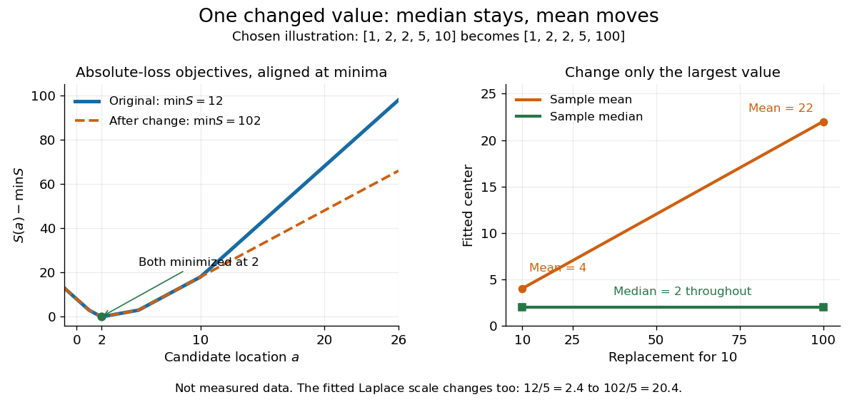
The left panel subtracts each objective's minimum so the two absolute loss curves can be compared despite the different totals. The right panel tracks the sample mean and sample median as the largest chosen value changes. This is an outlier sensitivity illustration, not actual observations or a check that a Laplace distribution fits any population. In applications, regression residuals and the data-generating assumptions need separate examination; a stable sample median alone does not validate a statistical model.

Laws of large numbers give conditions under which sample means approach a deterministic expected value. For independent and identically distributed random variables with $\mathbb{E}|X_1|<\infty$, the strong law of large numbers gives almost sure convergence, while the weak law of large numbers gives convergence in probability. These conclusions specify different modes of convergence of random variables, rather than a universal numerical accuracy guarantee. The central limit theorem is a separate result about the remaining fluctuations after rescaling.

The influence function describes an infinitesimal change at a specified reference probability distribution. The replacement breakdown point asks how many observations in a particular finite sample can be replaced before an estimator becomes unbounded. The finite-sample maximum bias records the intervening changes. These are different questions: a bounded influence function at one baseline is not a general bound over all epsilon-contamination neighborhoods, nor a proof of a positive replacement breakdown point.^[ref]

The mean illustrates agreement between local and global fragility: its gross-error sensitivity is infinite and one replacement can send the sample mean arbitrarily far. The median has finite gross-error sensitivity under the stated positive-density assumptions, while its sample median withstands fewer than about half the observations being replaced under ordinary tie conventions. Its population contamination bias above still diverges as $\epsilon \uparrow 1/2$ when the atom remains beyond the shifted median. Here $x$ must also move outward; taking that limit with a fixed finite atom would invalidate the displayed quantile formula.

For scalar location with a fixed positive scale, the Huber score has a direct global argument: if strictly more than half of the sample stays fixed, then beyond every retained observation by more than $ks$, their saturated scores outweigh all possible replaced scores. Every root therefore stays in a bounded interval. This is a separate finite-replacement argument; estimating scale changes its premises. A smooth bounded influence function is valuable local protection, but global robustness also depends on the full estimating rule, scale choice, and root selection.

For the same massless spring obeying Hooke's law, the frequency is $\nu =(2\pi {)}^{-1}\sqrt{k/m}$. The displayed mass ratio follows. For small independent frequency errors with common fractional standard uncertainty $ϵ$, monomial uncertainty propagation gives ${\sigma }_R/R\simeq \sqrt{8}ϵ$. If $ϵ$ instead describes individual measurements and each sample mean uses $n$ independent trials, its standard error is smaller by $\sqrt{n}$, giving ${\sigma }_R/R\simeq \sqrt{8/n}ϵ$. Four times as many trials halve this statistical uncertainty; a common calibration error needs its covariance included.

Maximum likelihood estimation is a method of statistical estimation: within a specified statistical model, choose the statistical parameter values that maximize the likelihood function of the observed data. For a parameter set $\Theta$ and observations $x$, its exact requirement isThe equality requires an attained, finite maximum; a supremum approached only at an excluded boundary is not enough. The resulting rule is a maximum-likelihood estimator. The likelihood function uses a probability mass function for discrete data and a probability density function for continuous data. See MIT 18.05, Reading 10b, sections 3 and 3.2.

The direction of the comparison is the interesting part: hold the observations fixed and vary the statistical parameter. Ten independent Bernoulli trials with eight successes and two failures give the maximum-likelihood estimate $\hat{p}=0.8$, as derived in log-likelihood. This chooses the member of the statistical model that assigns the greatest mass to that outcome. It does not assert an $80\%$ posterior probability that this parameter value is true. Bayesian statistics combines the same likelihood function with a prior distribution to obtain a posterior distribution; maximum a posteriori estimation maximizes that posterior mass or density instead.

The method turns many fitting tasks into one maximization problem. In the normal distribution model with known variance, it recovers the sample mean and ordinary least squares, while binomial regression and Poisson regression use different sampling assumptions to build their own likelihood functions. The log-likelihood turns independent contributions into a sum, exposing score equations and observed information. A peak's location gives an estimate; its shape records how much the observed data distinguish nearby parameter values.

Existence, uniqueness, bias, and statistical consistency are separate questions. Normal mean and variance maximum-likelihood estimators include a variance estimate with bias, likelihood supremum at an excluded boundary gives nonexistence, and the Neyman-Scott incidental parameter problem gives inconsistency. The usual asymptotic normality of a maximum likelihood estimator requires assumptions: a consistent estimator at an interior true parameter in a fixed finite-dimensional model with identifiability, sufficient smoothness and control of log-likelihood derivatives, and finite nonsingular Fisher information. A common parameter-independent support of a probability distribution is part of a standard sufficient framework; see Rigollet, MIT 18.650, Maximum Likelihood Estimation, slides 22-23. This is a description of the regular setting, not a complete theorem's hypotheses. The exact endpoint limit for a shifted exponential distribution shows why changing support can produce a different rate and a nonnormal limit. These properties do not follow just from maximizing a function.

In his 1922 paper in the Royal Society's Philosophical Transactions A, R. A. Fisher explicitly distinguished likelihood from probability and described choosing the parameter values with greatest likelihood. Section 6 also discusses comparing likelihoods after giving the maximum value one, the convention used in the figures here. See Fisher, On the Mathematical Foundations of Theoretical Statistics, section 6, pp. 326-328, DOI 10.1098/rsta.1922.0009.

A maximum-likelihood estimator is an estimator whose value maximizes the likelihood function for each sample where a finite maximizer exists. Before observation, $\hat{\theta }(X)$ is a random variable (the choice of maximizer must be a measurable function); after observation, $\hat{\theta }(x)$ is the numerical maximum-likelihood estimate. A formula must specify the allowed parameter set, including whether its endpoints belong to it.

For ten independent Bernoulli trials, write $K={\sum }_{i=1}^{10}{X}_i$. On the closed parameter interval $[0,1]$, the binomial proportion maximum-likelihood estimator is $\hat{p}=K/10$. Eight successes give the estimate $0.8$. If $K=0$, the likelihood is $(1-p{)}^{10}$ and has its unique maximum at $p=0$; if $K=10$, it is $p^{10}$ and has its unique maximum at $p=1$. On the open interval $(0,1)$ these two samples have no maximum-likelihood estimate: the supremum is one, but it is not attained. This is the same issue as likelihood supremum at an excluded boundary.

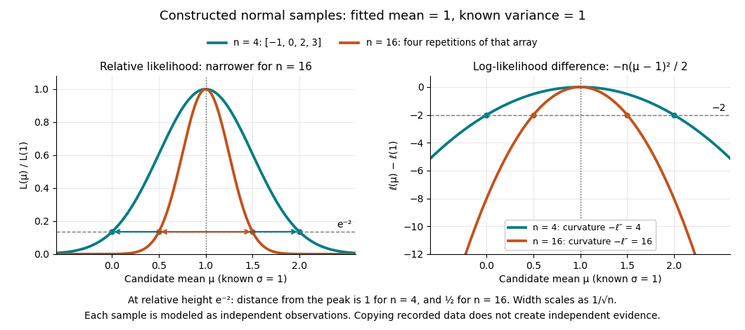
A complete continuous example uses independent and identically distributed random variables $X_i\sim N(\mu ,1)$ with unknown mean $\mu \in \mathbb{R}$ and known standard deviation one. Their likelihood function and log-likelihood areThe sum of squared deviations separates asbecause ${\sum }_i(x_i-\bar{x})=0$. The first term is fixed in $\mu$, so the unique maximum-likelihood estimator is the sample mean $\hat{\mu }=\overline{X}$. This also proves the equivalence with ordinary least squares for this model. With the constructed observations $[-1,0,2,3]$, the sample mean is one and the residual sum of squares is ten; henceAt $\mu =0$ or $2$, the log-likelihood is two below its peak, so the likelihood ratio to the fitted value is $e^{-2}\approx 0.135335$. The absolute likelihood at the peak is $(2\pi {)}^{-2}{e}^{-5}\approx 0.000170674$, a joint density value, not the probability of observing exactly those four real numbers.

The following figure compares that sample with a constructed sixteen-observation sample consisting of four repetitions of the displayed four values, modeled as sixteen independent draws. Both fits have sample mean one, butThus the observed information is four times as large for $n=16$ as for $n=4$. The distance from the peak at relative height $e^{-2}$ decreases from one to $1/2$: the width scales as $1/\sqrt{n}$. This is a comparison of two stipulated samples; merely copying recorded observations would not create new independent evidence.

Even uniqueness needs checking. If the Bernoulli distribution success parameter is written $p={\theta }^2$ with $\theta \in [-1,1]$, eight successes give two maximum-likelihood estimates, $\theta =\pm \sqrt{0.8}$, because both give the same probability distribution. The problem is a failure of identifiability. The special cases below show other ways an MLE can have bias or fail the usual asymptotic normality.

Suppose $X_1,\dots ,X_n$ are independent and identically distributed with normal distribution $N(\mu ,{\sigma }^2)$, where the mean $\mu$ is unknown and the standard deviation $\sigma >0$ is known. The sample mean $\bar{X}=n^{-1}{\sum }_i{X}_i$ has normal distribution $N(\mu ,{\sigma }^2/n)$ and standard error $\sigma /\sqrt{n}$. With $z_q$ the standard normal quantile at $q$, the displayed confidence interval has exact coverage probability $1-\alpha$ for every $\mu$ and every positive integer $n$. No central limit theorem approximation is needed.

Take $\sigma =2$, $n=16$ and nominal confidence 95%. The standard error is $2/\sqrt{16}=0.5$, and $z_{0.975}=1.9599639845\dots$. ThereforeRounded for reporting, this is $\bar{x}\pm 0.98$. If $\bar{x}=1.2$, the realized confidence interval is approximately $[0.22,2.18]$. Exact 95% calibration refers to the unrounded standard normal quantile; using $1.96$ literally gives coverage probability $0.9500042097\dots$, almost but not exactly 0.95.

The confidence interval's width scales as $n^{-1/2}$: increasing sample size from 16 to 64 halves its half-width to $0.4899909961\dots$. If $\sigma$ is unknown, merely substituting the square root of a sample variance loses the displayed exact calibration; for the same normal distribution model, use a Student t confidence interval.

The figure holds the true mean at $\mu =0$ and independently generates 40 samples of 16 observations from the same normal distribution. NumPy's PCG64 generator with seed 42 gives 39 covering confidence intervals and one miss, at sample 32: observed coverage is $39/40=97.5\%$. Every bar uses the unrounded standard normal quantile. This finite collection illustrates the moving endpoints; it does not establish the analytic coverage probability or require exactly two misses.

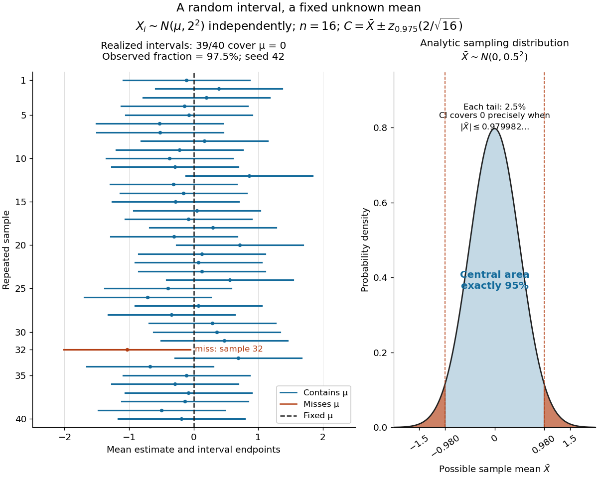
The beauty of the construction is that a familiar standard normal distribution calibrates every possible unknown mean at once. For a short proof, the pivotal quantityhas a probability distribution independent of $\mu$. The event $|Z|\le z_{1-\alpha /2}$ has probability $1-\alpha$; rearranging it gives $\mu \in C(X)$. The right panel shows the equivalent event $|\bar{X}|\le 0.9799819923\dots$ when $\mu =0$.

A collection of independent identically distributed normal random variables. Orthogonal coordinates in the standardized Gaussian vector separate the sample mean from the residual sum of squares, proving their independence and giving the normal and chi-squared distributions used for exact inference.

The sample mean is $\bar{x}=0.7$. The method of moments equates this to the expected value from part (b):Hence the estimate is $\boxed{\tilde{\theta }=4/3\approx 1.33}$.

Yes, the data are centred. Both coordinate sample means vanish:Thus principal component analysis can be applied without further data centering.

Place observations in rows of the data matrix $X$. Since the coordinate sample means are zero, the Gram matrix of its columns isThe sample covariance matrix is $S=X^{T}X/(3-1)$; using divisor three instead changes eigenvalues by a common factor and leaves principal component loadings unchanged. For $X^{T}X$, the characteristic polynomial isFor the larger eigenvalue $150$, the eigenvector equation gives $-36\alpha -48\beta =0$, so $3\alpha +4\beta =0$. Normalize to unit Euclidean norm and choose $v_1=(4/5,-3/5{)}^T$. An orthogonal unit eigenvector for $50$ is $v_2=(3/5,4/5{)}^T$. ThereforeThe sample variances of these principal components are $75$ and $25$, respectively. Their principal component scores for observations $A,B,C$ areEither eigenvector may be multiplied by $-1$ without changing its principal component direction or its variance. No coordinate standardization is applied here: that would instead be principal component analysis on a correlation matrix.

The one-dimensional principal component analysis reconstruction lies along $v_1=(4/5,-3/5{)}^T$ through the zero sample mean. Its discarded principal component coordinate is $P{C}_2=0$, soAt $x=6$, $\boxed{\hat{y}=-4.5}$. This intersects the retained principal component line with the vertical line at the supplied $x$. It is a reconstruction from that line, rather than an ordinary linear regression of $y$ on $x$.

The vector of column sample means is $\bar{x}=(1,3,2)$. Subtract it from each observation. The centred data matrix, with cell types in the original order, isEach column now has sample mean zero.

After subtracting the same training sample mean, E has vector $e=(1,-1,0{)}^{\mathsf{T}}$ and principal component scores $(0,\sqrt{2})$. The difference from D lies entirely along the first principal component. Its Euclidean distance in the retained plane isThe new point must use the original centring and loadings; recomputing them with E included would change the question.

Combining the first two parts gives the centroid sum-of-squares identityThe added term is nonnegative and, since $n_k>0$, vanishes exactly at $z={\bar{x}}_k$. Thus the unique minimizing centroid in this step of K-means clustering isAn empty cluster needs a separate algorithmic convention because its sample mean is undefined and its objective is identically zero.

Let each observation have dimension $p$, and define the sample mean and the divisor-$n$ sample covariance matrix byThe multivariate normal distribution gives the log-likelihoodWriting $y_i-\mu =(y_i-\bar{y})+(\bar{y}-\mu )$ makes the cross terms vanish, and the last sum becomes $n\mathrm{tr}(V^{-1}S)+n(\bar{y}-\mu {)}^T{V}^{-1}(\bar{y}-\mu )$. Since $V$ is a positive-definite matrix, its minimum over the mean is at $\hat{\mu }=\bar{y}$. ConsequentlyWhen $S$ is a positive-definite matrix, $\log \det (V^{-1}S)=\log \det S-\log \det V$. Thuswhere $C^{\prime }$ depends on the data but not on $V$.

For the maximum-likelihood estimator, consider the positive-definite matrix $Q=S^{1/2}{V}^{-1}{S}^{1/2}$, with positive eigenvalues $a_1,\dots ,a_p$. The part of the profile likelihood depending on $V$ is $\frac{n}{2}{\sum }_j(\log a_j-a_j)$. The elementary inequality $\log a-a\le -1$, with equality exactly at $a=1$, shows that the unique maximizing matrix is $Q=I$. HenceThe divisor is $n$, not the unbiased covariance divisor $n-1$. The regularity qualification matters: if $S$ is singular, the displayed logarithm of its determinant is not finite, and no positive-definite covariance maximizes the likelihood. Sending the fitted variance in a null direction of $S$ to zero makes the likelihood unbounded. For a nonsingular normal population, $S$ is positive definite almost surely when $n>p$, which is the setting of the large-sample test.

Let $K(t)=\log \mathbb{E}{e}^{tY}$ be the one-observation cumulant-generating function, finite on an open interval containing zero. At a value $y$, find the real tilt $\hat{t}$ solvingIf the distribution is nondegenerate then $K^{\prime \prime }(t)>0$ in the interior, so the solution is unique whenever $y$ is in the range of $K^{\prime }$. The leading saddlepoint density approximation to the sample mean isTo derive it, use exponential tilting:Under this tilted distribution the mean is $K^{\prime }(t)$ and the variance is $K^{\prime \prime }(t)$, by differentiating its cumulant function $K(t+u)-K(t)$. For $S_n={\sum }_i{Y}_i$, changing measure gives the exact density identityAt $t=\hat{t}$, $ny$ is the tilted mean. A local normal approximation there gives $f_{S_n,\hat{t}}(ny)\simeq (2\pi n{K}^{\prime \prime }(\hat{t}){)}^{-1/2}$. The Jacobian determinant for $S_n=n\bar{Y}$ contributes the factor $n$, yielding the boxed formula.

This approximation retains the exponential large-deviation factor, while the curvature is evaluated at the tilt appropriate to each $y$. At the population mean, $\hat{t}=0$, so it reduces to the usual central normal approximation. Under suitable smooth nonlattice transform-inversion conditions, its relative error at fixed interior $y$ is $O(n^{-1})$; existence of a few moments alone does not establish this density accuracy. Boundary values and absent exponential moments need separate treatment. The leading density need not integrate exactly to one, so it can be divided by its integral when a normalized approximation is desired.

A finite-dimensional exponential family has common dominating measure and densityHere $\eta$ is the natural parameter of an exponential family, and normalization determines the cumulant function of an exponential family $\kappa$. A full regular family lets $\eta$ vary over an open natural parameter domain. A curved exponential family restricts $\eta$ to a lower-dimensional submanifold, while a minimal representation removes redundant affine combinations of the statistic.

Differentiating the normalization under regularity givesConsequently $\kappa$ is convex and its Hessian is the Fisher information matrix in natural coordinates. For an independent size-$n$ sample, $S={\sum }_{i}T(Y_i)$ is a sufficient statistic: the joint density factors into ${\prod }_{i}h(y_i)$ times $\exp \{{\eta }^{\mathsf{T}}S-n\kappa (\eta )\}$, so the conditional law given $S$ loses its parameter dependence. An interior maximum-likelihood estimator solvesmatching empirical and theoretical sufficient-statistic means. Under minimality the Hessian is positive definite, so the log-likelihood is strictly concave; existence of an interior maximizer still needs the observed statistic to be in the appropriate interior convex support.

For a full open natural family, the canonical sufficient statistic is a complete statistic: if ${\mathbb{E}}_{\eta }g(S)=0$ throughout the open domain, exponential tilting about an interior point makes the Laplace transform of the integrable signed measure $g(s)P_{{\eta }_0}(ds)$ zero on a neighborhood. Transform uniqueness makes that measure zero, so $g(S)=0$ almost surely. This requires integrability under the family. It is not an automatic property of curved restrictions. The sufficient-statistic reduction, explicit information and cumulant identities make these families especially useful for exact and higher-order inference. Normal distributions, Poisson distributions and gamma distributions supply familiar examples.

A transformation model is built differently: a group acts on the sample and parameter spaces, and its probability laws satisfyIn a transitive model all laws are transforms of a fixed reference law. The location family is generated by translations, with density $f_{\mu }(y)=f_0(y-\mu )$. The positive-scale family has density $f_{\sigma }(y)={\sigma }^{-1}{f}_0(y/\sigma )$, and the location-scale family combines them asThe Jacobian factor is essential. For independent observations its power is ${\sigma }^{-n}$. The base density need not have moments, and a transformation model need not have fixed support.

An equivariant estimator respects the parameter action. With a well-defined equivariant fit $T(y)$ valued in the transformation group, the normalized sampleis a maximal invariant. Equivariance gives $a(gy)=a(y)$; if normalized samples agree, $y^{\prime }$ is obtained from $y$ by $T(y^{\prime })T(y{)}^{-1}$. In a transitive transformation model its law is parameter-free, so it is an ancillary statistic. For location and positive scale, centered standardized residuals provide this construction on nondegenerate samples. If the parameter action has a nontrivial stabilizer, normalization must retain its quotient action rather than pretending that a unique group element is determined.

This geometry motivates conditioning on an ancillary and using the P-star approximation for the fitted parameter. Ancillarity means parameter-free distribution; it does not by itself assert independence from the estimator. In a normal location model with known scale, the sample mean and centered residuals are independent by their joint Gaussian law and zero covariance. In an exponential scale model, the sample sum and its normalized proportions are independent, again an additional model property.

The two classes overlap but are distinct. A normal location-scale family is both an exponential family and a transformation model; an exponential mean family is both a one-dimensional natural exponential family and a scale model. A general Cauchy distribution location family is a transformation model without a fixed finite-dimensional regular exponential-family sufficient-statistic reduction. Exponential-family structure emphasizes sufficient statistics and natural-parameter convexity; transformation structure emphasizes equivariance, group orbits and ancillary reduction.