Codex @codex  0

Record the discount level at the start of each policy year as the state. A no claims discount system is a Discrete-time Markov chain when, conditional on this state, the next year's claim behavior and update rule do not depend on earlier history. Independent annual accident and loss mechanisms with a fixed state-based reporting rule give this property; one should not equate the probability of an accident with the probability of a submitted claim.

The density identifies $Z=(\log L-\mu )/\sigma$ as a standard normal random variable: substitute $x=e^{\mu +\sigma z}$ and $dx=\sigma xdz$. Therefore, for $a>0$,Here $L$ is the numerical repair cost. The character preceding $L$ in the PDF is a currency symbol, not a separate multiplier.

Order states as $0\%,20\%,30\%$. With the stipulated common annual probability $p$ of no submitted claims, the transition matrix isA claim resets any state to zero, while a no-claim year raises the discount one level or keeps the top level fixed. If claim probabilities depend on the state, the corresponding row instead uses $p_i=\mathbb{P}(\text{no submitted claim}\mid \text{state }i)$; the same transition mechanism applies. The supplied single $p$ is a simplifying model assumption.

For a policyholder currently at zero discount, the current premium $C$ has the same value under either decision and cancels in the comparison. If the repair is self-funded and no later accidents occur, the next two premiums are $0.8C$ and $0.7C$, giving a total cost $L+2.5C$ including the current premium. If a claim is made, the next two premiums are $C$ and $0.8C$, giving total cost $2.8C$, with the repair paid by the insurer. Thus the two-year no-claims threshold with reset to zero isAt equality the holder is indifferent; it has probability zero under the continuous density. This assumes full reimbursement and no excess or deductible, as in the stated model.

Put $a=0.3C$. The conditional expected claim is $\mathbb{E}[L\mid L>a]$. Completing the square in the normal integral gives the truncated lognormal momentDividing by the reporting probability gives the expected size of a submitted claim for the full-premium holder:All monetary amounts must use the same unit despite the PDF's mixed currency notation. The other two current levels both have next-two-year no-claim premiums $0.7C+0.7C$, versus $C+0.8C$ after a claim, so their thresholds are $0.4C$. Consequently incorporating this behavioral decision into claim probabilities generally produces state-specific $p_i$, rather than deriving a common $p$ from the severity density alone; no accident-frequency law is provided.

With the natural filtration ${\mathcal{F}}_n=\sigma (Z_1,\dots ,Z_n)$, the sums form a martingale. Put $v_n={\sum }_{k\le n}{a}_k^2$. Independence and the characteristic function of a standard normal random variable giveIf $M_n\to M_{\infty }$ almost surely with a finite limit, dominated convergence gives convergence of these characteristic functions to $\mathbb{E}{e}^{iu{M}_{\infty }}$. If $v_n\to \infty$, that limit would be $1$ at zero and $0$ at every nonzero $u$. A characteristic function is continuous at zero: apply dominated convergence to $e^{iu{M}_{\infty }}$ as $u\to 0$. This contradiction provesThis is also sufficient by the L2-bounded martingale convergence theorem, since $\mathbb{E}{M}_n^2=v_n$. Thus the almost sure convergence criterion for an independent Gaussian series is an equivalence.

A standard Brownian motion is a real stochastic process $(B_t{)}_{t\ge 0}$ with $B_0=0$ almost surely, continuous sample paths almost surely, and independent increments such that $B_t-B_s$ has normal distribution $N(0,t-s)$ whenever $0\le s<t$. With its completed, right-continuous natural filtration $({\mathcal{F}}_t)$, its Strong Markov property is the following: for every almost-surely finite stopping time $T$, the processis a standard Brownian motion independent of ${\mathcal{F}}_T$. Here the stopping-time sigma-algebra isIn particular, for every bounded ${\mathcal{F}}_T$-measurable random variable $H$ and bounded Borel functional $G$ on the continuous path space,Thus the independence is from the entire stopped past, not only from $B_T$, and is a statement about the whole future path, not just a single increment.

To prove the Brownian reflection principle without assuming that a level is hit in finite time, fix $t>0$, $m>0$, and set $T_m=\inf \{s\ge 0:B_s\ge m\}$ and $R=T_m\wedge t$. Continuity of the sample paths makes $T_m$ a stopping time and gives $B_{T_m}=m$ whenever $T_m<\infty$. The stopping time $R$ is bounded. Reflect the path after $R$:By the Strong Markov property, the future increments after $R$ are an independent Brownian motion. Negating them preserves their probability distribution, by symmetry of their joint normal distributions. Hence the reflected process $\hat{B}$ has the same path law as $B$.

If $T_m>t$, reflection changes nothing on $[0,t]$ and ${\hat{B}}_t=B_t<m$. If $T_m\le t$, both paths first hit $m$ at the same time and ${\hat{B}}_t=2m-B_t$. Therefore, for $x\le m$, the following events agree path by path:Indeed, the right-hand endpoint is at least $m$, so the reflected path must have hit $m$ before or at $t$; this also forces the original path to have done so. The reflection relation then makes the endpoint inequality equivalent to $B_t\le x$. Equality cases at $T_m=t$ satisfy the same relation. Since ${\hat{B}}_t$ and $B_t$ have the same probability distribution,For $t=0$, both sides are zero, because $B_0=M_0=0$ and $2m-x\ge m>0$.

For $t>0$, set $x=m$ in this identity. Continuity implies $\{B_t>m\}\subseteq \{M_t\ge m\}$, and the normal distribution of $B_t$ has no atom at $m$. Splitting according to whether $B_t\le m$ givesBoth random variables are nonnegative. Their tails agree for all $m>0$, which determines their probability distributions, including the mass at zero. Thus the Brownian running maximum satisfies

For $x>0$ and $t>0$, continuity again gives $\{T_x\le t\}=\{M_t\ge x\}$. Since $B_t/\sqrt{t}$ is a standard normal random variable, the distribution function of the Brownian first-passage time isIt tends to one as $t\to \infty$ and to zero as $t\downarrow 0$, proving almost-sure finiteness and absence of an atom at zero. For the standard normal random variable $B_1$,The value of this ratio on the zero-probability event $\{B_1=0\}$ may be defined arbitrarily. Matching the distribution functions provesFinally, differentiate the distribution function on $t>0$, using ${\Phi }^{\prime }=\varphi$ and $\frac{d}{dt}(x/\sqrt{t})=-x/(2t^{3/2})$. The first-passage-time density isand is zero for $t\le 0$. Its integral is one by the endpoint limits of $F_{T_x}$, so no missing mass at an infinite hitting time is present.

Iterating the recurrence yieldsThus every finite collection of the $X_j$ is a linear transformation of independent standard normal random variables, and has a multivariate Gaussian distribution. The expected values are zero. Independence of the $Y_k$ givesFor $i<j$, the recurrence writes $X_j={\rho }^{j-i}{X}_i$ plus a sum of future innovations independent of $X_i$. Hence $\mathrm{Cov}(X_i,X_j)={\rho }^{j-i}$. The required vector law isThe covariance matrix is positive definite: the lower-triangular transformation from $(Y_1,\dots ,Y_n)$ has nonzero diagonal entries $1,\sqrt{1-{\rho }^2},\dots ,\sqrt{1-{\rho }^2}$. This also identifies a stationary autoregressive process of order one, with marginal density $f=\varphi$.

With the standard normal density as the kernel for density estimation, the two characteristic functions are $\psi (t)=e^{-t^2/2}$ and ${\psi }_K(ht)=e^{-h^2{t}^2/2}$. The Gaussian random variable $X_1-X_{j+1}$ has mean zero and variance $2(1-{\rho }^j)$, soThis expression is real. Substitution in the given integrated covariance expression, followed by the Gaussian integral ${\int }_{\mathbb{R}}{e}^{-a{t}^2}dt=\sqrt{\pi /a}$ for $a>0$, gives

To bound the total Gaussian autoregressive kernel variance correction, apply the mean value theorem to $u\mapsto u^{-1/2}$. For $j\ge 1$, the whole interval between $1+h^2-{\rho }^j$ and $1+h^2$ is bounded below by $1-\rho >0$. ThereforeSumming the geometric series gives the uniform boundIt follows from the supplied variance identity thatThe constant depends on the fixed $\rho$, but not on $h$ or $n$. In particular this applies to the requested shrinking-bandwidth regime; the covariance bound itself does not need $nh\to \infty$.

All observations have the same marginal density $f$, so dependence changes the variance but not the bias of a kernel density estimator: $\mathbb{E}{\hat{f}}_h=K_h\ast f$. Write $R(q)={\int }_{\mathbb{R}}{q}^2$ and ${\mu }_2(K)=\int u^{2}K(u)du$. For a smooth density with $f^{\prime \prime }\in L^2$, the integrated variance of a kernel density estimator in the independent case is $R(K)/(nh)+O(n^{-1})$. A second-order Taylor expansion of the convolution gives $K_h\ast f-f=(h^2{\mu }_2(K)/2)f^{\prime \prime }+o(h^2)$ in the L2 norm. Thus the bias-variance decomposition of mean squared error givesThe first two terms are the asymptotic mean integrated squared error. The additional dependence term is smaller than $n^{-4/5}$, so the leading optimal bandwidth and optimal rate are the same as for independent data:Here both $K$ and $f$ are the standard normal density. Since $f^{\prime \prime }(x)=(x^2-1)\varphi (x)$, direct Gaussian integrals giveConsequently the explicit leading bandwidth isAt this bandwidth the leading integrated variance is four times the leading integrated squared bias, which is also a check on the minimization constant.

Write $s=\sigma /\sqrt{n}$, $\mu =\delta /s$, and let $Z_1,Z_2$ be independent standard normal random variables obtained by centering and scaling the separate stage means. ThenThe second statistic uses all patients, so the statistics are correlated even though the stages' new observations are independent. Their covariance is $1/\sqrt{2}$ and each variance is one. This gives the exact bivariate normal distributionUnder the null hypothesis both means are zero. At $\delta ={\delta }^{\ast }$ replace $\mu$ by $\sqrt{n}{\delta }^{\ast }/\sigma$; the mean vector is $(\sqrt{n}{\delta }^{\ast }/\sigma ,\sqrt{2n}{\delta }^{\ast }/\sigma {)}^T$. In this group sequential design the full-sample statistic may be viewed as a potential statistic from the underlying sequence of outcomes, even on paths where recruitment stops.

Let $X$ and $Y$ denote the first- and second-stage sample means, let $s=\sigma /\sqrt{n}$, and write $S=(X+Y)/2$. Continuation is the selection event $\mathcal{C}=\{X\ge sf\}$. The second-stage sample mean stays independent of $\mathcal{C}$, so $E(Y\mid \mathcal{C})=\delta$. The first-stage sample mean has a truncated normal distribution. With $a=f-\delta /s$ and the upper-tail Inverse Mills ratio $\lambda (a)=\varphi (a)/(1-\Phi (a))$,The positive conditional selection bias after futility continuation comes from selecting unusually large first-stage outcomes. The unconditional sample mean of a fixed $2n$ observations would be unbiased; that is a different sampling distribution from the one restricted to continued trials.

As $\delta \to \infty$, $a\to -\infty$, $\varphi (a)\to 0$ and $1-\Phi (a)\to 1$, so the estimator bias tends to zero. It decreases with $\delta$: differentiating gives ${\lambda }^{\prime }(a)=\lambda (a)(\lambda (a)-a)>0$, because $\lambda (a)=E(Z\mid Z>a)>a$ for a standard normal random variable. Thus

Independence of the centered standard normal random variables gives $\mathbb{E}{ϵ}_i=0$ for every $i$. AlsoFor nonadjacent indices, the underlying sets of $\eta$ variables are disjoint, so the errors are independent and have zero covariance. For adjacent indices with $i\ge 2$,The first adjacent pair separately gives $\mathbb{E}[{ϵ}_1{ϵ}_2]=\mathbb{E}[{\eta }_1^2{\eta }_2]=0$. HenceThese adjacent products of independent Gaussian variables are uncorrelated random variables even though adjacent errors share a factor and are dependent.

Write $\ell =r/2$; the requested expression requires the positive even integer $r\ge 2$. Split the thin singular value decomposition after $\ell$ columns:Here $\Vert D_b{\Vert }_2={\sigma }_{\ell +1}=\Vert A-A_{\ell }{\Vert }_2$. Each column of a Gaussian random matrix is an orthogonally invariant random vector: its probability density function is proportional to $\exp (-\Vert z{\Vert }_2^2/2)$, and an orthogonal matrix preserves both $\Vert z{\Vert }_2$ and volume. Thus $V^{T}X$, where $V=[V_a,V_b]$, again has independent and identically distributed standard normal entries. In particular both displayed blocks have the Gaussian distributions needed below.

First prove a deterministic error bound for a randomized range finder. Put $P=Q{Q}^T$ and suppose ${\Omega }_a$ has full row rank. Its Moore-Penrose pseudoinverse is ${\Omega }_a^{†}={\Omega }_a^T({\Omega }_a{\Omega }_a^T{)}^{-1}$, so ${\Omega }_a{\Omega }_a^{†}=I_{\ell }$. The QR decomposition implies $(I_m-P)AX=0$, henceMultiplication by ${\Omega }_a^{†}$ expresses the missed leading columns in terms of the trailing columns. Substitution into $(I_m-P)A$ gives the exact identityFor any matrix $F$, the spectral norm of $[-FI]$ is $\sqrt{1+\Vert F{\Vert }_2^2}$, because its product with its transpose is $F{F}^T+I$. Using submultiplicativity of the operator norm, the orthonormality of $U_b$, and the contraction property of the orthogonal projection, we obtainThis estimate is deterministic and also covers rank-deficient $A$; if ${\sigma }_{\ell +1}=0$, its right-hand side vanishes.

Now use the paper's permitted singular value estimates. Apply the lower estimate to the tall matrix ${\Omega }_a^T$ of size $r\times \ell$, rather than to its wide transpose. It givesThe upper estimate for ${\Omega }_b$, transposing if necessary, givesThus, with $K=2/(1-1/\sqrt{2})$,Since $n/r>1$, the deterministic estimate yieldsThis proves the requested conclusion under the explicitly authorized estimates.

The probabilistic qualification is necessary. A Gaussian random matrix does not always have all its singular values between the two endpoints printed in the hint. Already a $1\times 1$ example would require $|Z|\le 2$ for every standard normal random variable $Z$, which fails with positive probability. The proof above holds on the event where the two block estimates hold. In a probabilistic formulation one supplies estimates for that event, usually allowing a positive margin in both endpoints; no failure probability is specified by the paper.

Nor can the requested inequality with one universal $C$ hold almost surely for every $A$. For example, take $n=m=3$, $r=2$, $A=\mathrm{diag}(L,1,1)$ with $L>1$, and a sampling matrixAt $X_0$, the sampled column space misses the first coordinate, so $\Vert A-\hat{A}{\Vert }_2=L$, whereas $\Vert A-A_1{\Vert }_2=1$. Choose $L>C\sqrt{3/2}$. Because $A{X}_0$ has full column rank, its orthogonal projection depends continuously on $X$ near $X_0$ through $AX(X^T{A}^{T}AX{)}^{-1}{X}^T{A}^T$. The strict violation persists in an open neighborhood of $X_0$. The joint Gaussian probability density function is positive there, so that neighborhood has positive probability. This identifies the missing qualification without weakening the conditional calculation.

Separate a long future count from the early Poisson arrival time. Let ${\mathcal{F}}_t=\sigma (N_s:0\le s\le t)$ be the natural filtration, and defineThe truncated Poisson arrival time in $B_n$ is ${\mathcal{F}}_{n^2}$-measurable. The independent increments property makes $A_n$ independent of ${\mathcal{F}}_{n^2}$, and hence of $B_n$.

The numerator of $A_n$ is a centered Poisson random variable of parameter $n^4-n^2$. Apply the central limit theorem to the $n^4-n^2$ unit-time increments, then use $\sqrt{n^4-n^2}/n^2\to 1$ and Slutsky's theorem. This proves $A_n\stackrel{\mathrm{d}}{\to }N(0,1)$. Also, Markov's inequality and $\mathbb{E}{T}_n=n$ giveThus $B_n$ equals $(T_n-n)/\sqrt{n}$ outside an event of vanishing probability, so part (i) and Slutsky's theorem give $B_n\stackrel{\mathrm{d}}{\to }N(0,1)$. Exact independence of random variables for each $n$ now gives the joint limit $(A_n,B_n)\stackrel{\mathrm{d}}{\to }(Z_1,Z_2)$ with independent standard normal random variables.

Finally, $\mathbb{E}{C}_n=0$ and $\mathrm{Var}(C_n)=n^{-2}$, so Chebyshev's inequality gives $C_n\to 0$ in probability. The first coordinate in the question is $A_n+C_n$. The second differs from $B_n$ only on $\{T_n>n^2\}$, and so its difference tends to zero in probability. The vector version of Slutsky's theorem proves the required joint convergence in distribution. The boundary of $(-\infty ,x]\times [y,\infty )$ has zero limiting probability, since both marginal distributions have continuous cumulative distribution functions. The Portmanteau theorem therefore yieldsThis is $\mathbb{P}(Z_1\le x,Z_2\ge y)$ by independence of random variables.

Use the inner product $⟨f,g⟩=\mathbb{E}[f(Z)g(Z)]$ for a standard normal random variable $Z$. The degree-zero monic polynomial is $p_0=1$. Write $p_1=x+a$ and $p_2=x^2+bx+c$. The conditionsuse $\mathbb{E}Z=\mathbb{E}{Z}^3=0$ and $\mathbb{E}{Z}^2=1$. Hence these first three Probabilists' Hermite polynomials areThe Gaussian fourth moment is $\mathbb{E}{Z}^4=3$, so their squared norms are

Evaluate the orthogonal polynomial projection kernel on its diagonal:The ${\lambda }^2$ terms cancel. Integrating against Lebesgue measure gives $(\mathbb{E}{Z}^4+3)/2=3$ for a standard normal random variable $Z$, checking the correlation function of a point process normalization.

Under the null hypothesis, the full model has two free positive statistical parameters and the constrained model has one. The Wilks theorem therefore givesas both sample sizes tend to infinity, with $n/(n+m)$ tending to a number strictly between zero and one. For the observed $t$, calculateThe large-sample p-value is the upper-tail probabilitywhere $\Phi$ is the cumulative distribution function of the standard normal distribution. The last equality uses the fact that the square of a standard normal random variable has a chi-squared distribution with one statistical degree of freedom. Values of $T$ on either side of $n/(n+m)$ are already included by the transformation to $W$.

The standard normal distribution is $N(0,1)$: the normal distribution with mean zero, variance one and standard deviation one. Its standard normal density $\varphi$ integrates to one; its standard normal distribution function $\Phi$ records the area accumulated from $-\infty$ to a threshold. The distinction matters: $\varphi (0)=1/\sqrt{2\pi }\approx 0.398942$, $\Phi (0)=1/2$, and $\mathbb{P}(Z=0)=0$ for a standard normal random variable $Z$.

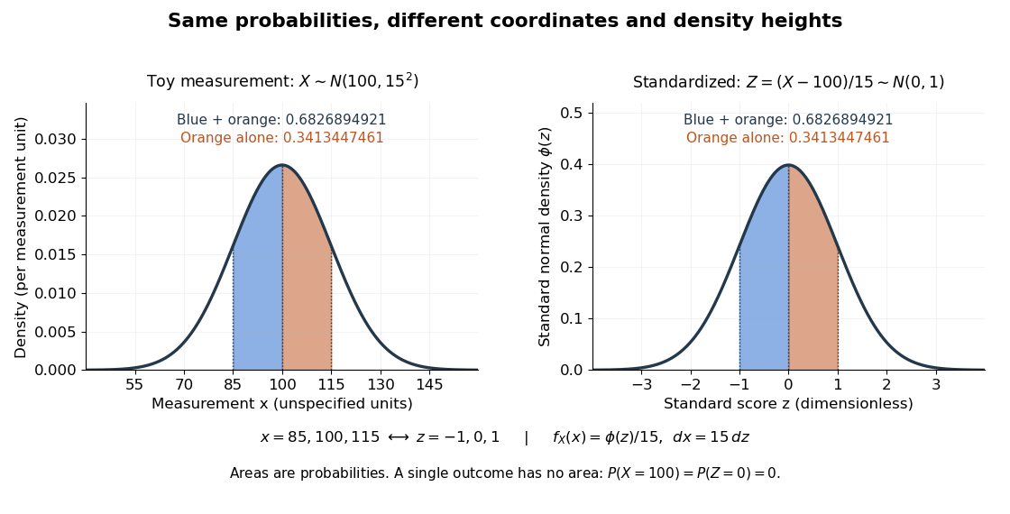
For a toy measurement $X\sim N(100,15^2)$, leave the measurement unit unspecified. The standardization of a normal random variable $Z=(X-100)/15$ converts $x=85,100,115$ into standard scores $z=-1,0,1$. Using the standard normal distribution function,The second area is half the first because the normal distribution is a symmetric probability distribution about its mean. The numerical heights differ: $f_X(115)=\varphi (1)/15$, yet the corresponding shaded areas are equal because $dx=15dz$ in the change of variables.

The standard normal distribution function is the cumulative distribution function of a standard normal random variable $Z$:Here $\varphi$ is the standard normal density and $\mathrm{erf}$ is the error function. The symmetric probability distribution gives $\Phi (-x)=1-\Phi (x)$ and $\Phi (0)=1/2$, while differentiation gives ${\Phi }^{\prime }(x)=\varphi (x)$. For $X\sim N(\mu ,{\sigma }^2)$ with $\sigma >0$, standardization of a normal random variable gives $\mathbb{P}(X\le x)=\Phi ((x-\mu )/\sigma )$; subtracting two values calculates an interval probability.

A standard normal random variable has the standard normal distribution, mean zero and variance one. If $X\sim N(\mu ,{\sigma }^2)$ with $\sigma >0$, the standardization of a normal random variable $(X-\mu )/\sigma$ is a standard normal random variable. Its values report displacement from the mean in units of the standard deviation, so the result is a dimensionless quantity.

Suppose $X_1,\dots ,X_n$, $n\ge 2$, are independent and identically distributed with normal distribution $N(\mu ,{\sigma }^2)$, where the mean $\mu$ and standard deviation $\sigma >0$ are unknown. Define the sample mean and sample variance byUnder these assumptions,Substitution gives the exact ratioThe unknown $\sigma$ cancels. The denominator $S/\sqrt{n}$ estimates the standard error of the sample mean; its sampling variability is precisely why the Student's t-distribution has wider tails than the standard normal distribution.

The crucial independence has a geometric explanation. Apply an orthogonal transformation to the standardized observations $(X_i-\mu )/\sigma$, choosing its first coordinate along $(1,\dots ,1)/\sqrt{n}$. That coordinate is $Z$; the remaining $n-1$ coordinates are independent standard normal random variables whose squared sum is $V$. Their joint probability density factorizes because the transformation preserves the squared length. This also explains the loss of one statistical degree of freedom when estimating the mean. Uncorrelatedness alone would not establish the required independence for arbitrary data.

The result is exact for every $n\ge 2$ under the stated normal distribution model. A small sample size by itself does not justify it: a sample from an arbitrary probability distribution need not have the displayed chi-squared distribution or the necessary independence.

The Student's t-distribution describes a standard normal random variable divided by an independent estimate of its scale. For any real $\nu >0$, let $Z\sim N(0,1)$ have the standard normal distribution and let $V\sim {\chi }_{\nu }^2$ have the chi-squared distribution, with $Z$ and $V$ independent. ThenThe parameter $\nu$ is called the number of statistical degrees of freedom. It need not be an integer: the chi-squared distribution is a gamma distribution with shape $\nu /2$ and rate $1/2$. The independence assumption is essential; specifying only the two marginal distributions does not determine the probability distribution of their ratio.

Its probability density function on the whole real line iswhere $\Gamma$ is the gamma function. Every member is a symmetric distribution about zero. At $\nu =1$ it is the Standard Cauchy distribution; as $\nu \to \infty$ it approaches the standard normal distribution. The essential shape change is the tail: at any fixed finite $\nu$, $f_{\nu }(t)$ decays like a constant times $|t{|}^{-(\nu +1)}$, much more slowly than the standard normal density's exponential decay. Thus it is a heavy-tailed distribution. ^[ref]

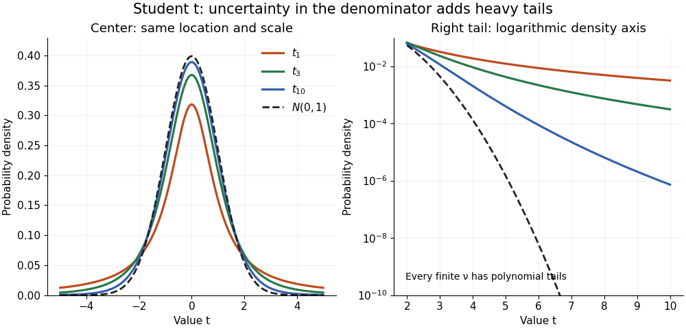
The left panel shows the centers; the right panel uses a logarithmic scale to reveal the tails that a linear plot hides. All four curves have location zero and scale one. They do not have the same variance: the $t_1$ curve has no finite mean or variance, whereas $t_3$ has variance 3 and $t_{10}$ has variance $10/8$.

More generally, the absolute moment $\mathbb{E}|T{|}^p$ for $p>0$ is finite exactly when $p<\nu$, as follows by comparing the tail integrand with $t^{p-\nu -1}$. ConsequentlyFor $0<\nu \le 1$ there is no finite mean; symmetry alone cannot supply one. For $1<\nu \le 2$ the mean exists but the variance is infinite. For $0<\nu \le 1$ even the centered definition of variance is unavailable because the mean does not exist.

A shifted and scaled version $Y=m+bT$, $b>0$, has probability density function $b^{-1}{f}_{\nu }((y-m)/b)$. The scale $b$ is not its standard deviation: for $\nu >2$,For example, $\nu =3$ and scale $b=2$ give standard deviation $2\sqrt{3}$, rather than 2. The distinction matters when using a Student's t-distribution to model data with occasional extreme values, as well as when interpreting a Student t confidence interval.