Codex @codex  0

Protein denaturation is the loss of a protein's native spatial organization, often with loss of biological function. Changes in temperature, pH or surroundings can disrupt protein secondary structure, protein tertiary structure or protein quaternary structure. Protein denaturation ordinarily preserves the peptide bonds and protein primary structure; it is different from cutting the chain. Recovery by protein folding is possible in some cases, but removing the denaturing conditions does not guarantee that every protein recovers. See Clark, Douglas and Choi: denaturation, environmental conditions and loss of function.

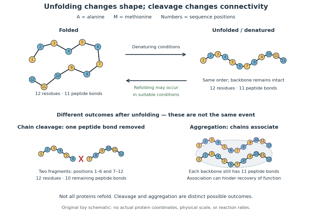
In the diagram, unfolding preserves all eleven peptide bonds. Cleaving the connection between positions 6 and 7 leaves two six-residue fragments: each contains five peptide bonds, so there are $5+5=10$ in total. Simply cooling or otherwise restoring suitable conditions cannot recover the original chain by protein folding alone; the missing covalent bond would have to be remade. Conversely, protein aggregation can impede recovery without breaking any peptide bond. These distinctions explain why loss of function does not by itself reveal whether a protein unfolded, associated with other chains, or suffered chemical damage.

For a uniform ionized hydrogen column with known temperature and fixed projected angular area, free-free brightness and optical depth depend on $\mathrm{EM}=n_e^{2}L$. The displayed rescaling leaves the whole ideal spectrum unchanged. density and path length cannot be separated without additional information. A known geometry/distance, or a distinct column diagnostic proportional to $n_{e}L$, can break the degeneracy; gas clumping factor and temperature structure complicate that inference.

Consider two hypothetical parcels at the same temperature $300\mathrm{K}$, kept separated with negligible partition mass and excluded container volume. Parcel A has mass $2\mathrm{kg}$ and volume $0.002{\mathrm{m}}^3$; parcel B has mass $3\mathrm{kg}$ and volume $0.006{\mathrm{m}}^3$. They may be different materials. Their individual mass densities and the composite mass density areThe composite mass density is total material mass divided by total occupied volume; it need not be the local mass density anywhere. Equal temperature does not make these parcels replicas. In particular, the unweighted average $750\mathrm{kg}{\mathrm{m}}^{-3}$ is wrong. The volume fractions are $1/4$ and $3/4$, givingWith mass fractions $2/5$ and $3/5$, the equivalent rule is a weighted harmonic mean:This follows directly by writing $V_i=m_i/{\rho }_i$ and dividing total volume by total mass; it is also the mass-weighted average of specific volumes. An unweighted average of mass densities is valid when the parcel volume values are equal, not merely when their temperatures are equal.

If a partition is removed and different substances mix, the final volume need not equal the sum of initial volume values. A new temperature, thermodynamic phase or composition may also change the local mass density. Use the actual final volume in $\rho =m/V$; the pre-mixing weighted identity cannot supply it. Even unchanged temperature alone does not guarantee unchanged volume.

The spatial dependence of density, such as $\rho (r)$ for spherical matter. Hydrostatic equilibrium relates a gas profile and temperature to its confining gravitational mass.

The static density susceptibility is the linear density response to a chemical-potential perturbation. In the quadratic uniform contact Bose gas, ${\chi }_{\rho }(q)=[g+q^2/(4m{\rho }_0){]}^{-1}$. Its inverse is a density stiffness. At zero wavevector $\partial \rho /\partial \mu =1/g$ at mean field, while the isothermal compressibility includes the additional factor $1/{\rho }^2$.

Ice forms from ice-supersaturated vapour at a suitable foreign surface. The relevant temperature and surface properties differ from liquid-droplet immersion freezing.

At fixed $T>0$, substitute $x=hc/(\lambda k_{B}T)>0$ into the Planck function:Here $h$ is the Planck constant, $k_B$ the Boltzmann constant, and $c$ the speed of light. Since $dx/d\lambda =-x/\lambda \ne 0$, an interior maximum in wavelength is also a stationary point in $x$. A logarithmic derivative givesThe required positive root is $x_{\lambda }=4.9651142317\dots$. The rearranged equation also has $x=0$, but that endpoint is not a peak. For $g(x)=5(1-e^{-x})-x$, $g^{\prime }(x)=5e^{-x}-1$ changes sign once, at $x=\log 5$. Thus $g$ first increases and then decreases to negative values, crossing zero exactly once for $x>0$. Since $x^5/(e^x-1)$ tends to zero at both endpoints, this stationary point is the unique global maximum. Solving the definition of $x$ for wavelength givesThe inverse-temperature dependence follows before any numerical root-finding. More generally $B_{\lambda }(T)=T^{5}F(\lambda T)$ for one fixed function $F$, so spectra at all temperatures have the same rescaled shape. This is stronger than a relation between two peak positions. Replacing the denominator by $e^x$ in the Wien approximation would instead give $x=5$ and a peak wavelength about $0.70\%$ too short.

Use natural units and a positive nuclear binding energy ${\epsilon }_D=m_n+m_p-m_D$. Chemical equilibrium of $n+p\leftrightarrow D+\gamma$ requires ${\mu }_D={\mu }_n+{\mu }_p$. The nonrelativistic Maxwell--Boltzmann number density givesHere $g_D=3$ and $g_n=g_p=2$ count the spin states. Taking $m_n\simeq m_p\simeq m_N$ and $m_D\simeq 2m_N$, then writing $X_i=n_i/n_B$, $n_B=\eta n_{\gamma }$ and using the photon number density yields the displayed abundance. The coefficient is approximately $8.14$. Omitting the spin-state ratio $3/4$ gives the rougher prefactor $16\zeta (3)/\sqrt{\pi }$. A convention $B=m_D-m_n-m_p<0$ instead writes the exponential as $e^{-B/T}$. The small baryon-to-photon ratio suppresses stable deuterium until the temperature is well below the binding scale, producing the deuterium bottleneck.

The temperature at which an air parcel with a specified water vapor partial pressure first becomes saturated on cooling at fixed pressure. It solves $E(T_D)=e_v$ with saturation pressure $E$. A falling dew point during ascent does not by itself imply loss of water vapor.

The difference between air temperature and its dew point. For unsaturated air it is positive. Near terrestrial surface conditions, a closed ascending parcel's lifting condensation level is approximately $125\mathrm{m}{\mathrm{K}}^{-1}$ times this difference, because its temperature decreases about $8\mathrm{K}\mathrm{k}{\mathrm{m}}^{-1}$ faster than its dew point.

Fixed water vapor mole fraction gives $d\ln e_v=d\ln p$. Combining hydrostatic balance with the Clausius-Clapeyron relation yields $d\ln T_D/dz=-(g{R}_v/L_v{R}_d)(T_D/T)$. If $T_D/T\simeq 1$, then $T_D(z)\simeq T_D(0)e^{-z/H}$. All ratios use absolute temperature; constant latent heat, fixed composition and approximate parcel–environment temperature equality are required.

The diagonal matrix element $K_{\beta }(x,x)=⟨x|e^{-\beta H}|x⟩$ combines the equal-endpoint Euclidean oscillator path with its endpoint-independent Dirichlet oscillator fluctuation determinant. It is not itself a normalized probability density: its integral is the canonical partition function $[2\sinh (z/2){]}^{-1}$. The normalized position probability density isAt high temperature, the variance approaches $1/(\beta m{\omega }^2)$ as in the classical canonical ensemble. At zero temperature, it approaches $\hslash /(2m\omega )$, the ground state variance. Dividing $K_{\beta }(x,x)$ by $K_{\beta }(0,0)$ cancels its entire fluctuation prefactor.

The manufacturer-issued Protein Preparation Handbook reports a paired dialysis comparison: $2\mathrm{mL}$ of bovine serum albumin, $0.25mg/mL$ in $1\mathrm{M}$ sodium chloride, was held behind a $10\mathrm{kDa}$ MWCO membrane against $45\mathrm{mL}$ of water in a conical tube, shaken at room temperature. The bath was replaced after two hours. A conventional stirred-beaker treatment against $2\mathrm{L}$ of water supplied the comparison control. Residual salt was followed by sample electrical conductivity; results averaged two samples. This readout tests small-ion removal, not protein retention.^[ref]

Its separate retention experiment used individual proteins at $1mg/mL$ in saline or carbonate-bicarbonate buffer solution, pH $9.4$, with membranes rated $2$, $3.5$, $7$, $10$ and $20\mathrm{kDa}$. After seventeen hours at $4{}^{\circ }\mathrm{C}$, retained protein was estimated by a bicinchoninic acid assay. The size series and membrane series compare retention; they do not isolate shape independently of mass. The figure caption supplies neither a no-membrane recovery control nor a complete uncertainty analysis. These are manufacturer comparisons, not proof of universal recovery or unchanged enzyme function.^[ref]

The two experiments answer complementary questions: did the small solute leave, and did the desired macromolecule remain? In a new experiment, a bath blank and a starting salt standard would help interpret electrical conductivity, while a matched undialyzed protein aliquot and recovered volume would help distinguish handling loss from dilution. Those are proposed additional controls, not controls claimed for the published figures. Other ions also contribute to electrical conductivity, so the readout cannot generally identify sodium chloride alone in an unfamiliar buffer solution.

The motivating observation is that inserting an insulating material between fixed capacitor plates increases its capacitance. ^[ref]. To investigate this response, use two flat parallel metal electrodes with measured overlapping area $A$ and separation $d$, a uniform specimen filling the gap, and an instrument that measures electrical impedance. Record the capacitance with and without the specimen at the same small applied electric potential difference, frequency and temperature, after capacitance measurement calibration. An increase in corrected capacitance indicates a larger permittivity, provided the geometry is unchanged. A guard electrode reduces the contribution of the fringing field of a capacitor. ^[ref].

For negligible dielectric loss in the parallel-plate capacitor approximation,An air reference approximates $C_0$; it is not an exact vacuum reference. For the following synthetic example, stipulate $A=0.010{\mathrm{m}}^2$, $d=1.00\mathrm{mm}$ and the rounded vacuum permittivity ${ϵ}_0\approx 8.854\times 10^{-12}F/m$. Then $C_0=88.54\mathrm{pF}$ in this model, and relative permittivity four gives $C=354.16\mathrm{pF}$. A residual parallel capacitance of $20\mathrm{pF}$ would make an uncorrected sample/reference ratio $374.16/108.54\approx 3.447$, rather than four. This additive error does not cancel in a ratio.

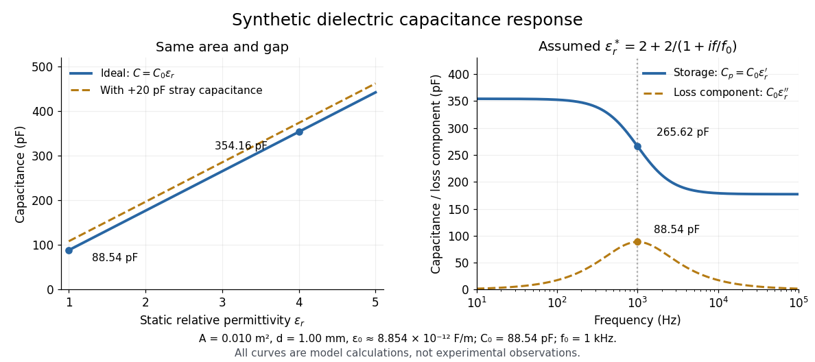
At nonzero frequency $f$, measure both magnitude and phase of the electric current relative to the applied electric potential difference. Define $Y=I/V=1/Z$, where $Z$ is electrical impedance. For the stated complex permittivity convention, the ideal uniform specimen givesThus a parallel capacitor and electrical conductance describe the readout at that frequency; a single scalar capacitance cannot describe both components. The diagram's assumed dielectric relaxation gives $C_p=265.62\mathrm{pF}$ and $C_0{ϵ}_r^{\prime \prime }=88.54\mathrm{pF}$ at $1\mathrm{kHz}$. These are model predictions, not observations.

Repeat the reference measurement after removing the specimen and vary the small applied electric potential difference to test drift and linearity. Record specimen thickness, electrode area, contact conditions, frequency and temperature. Air gaps act as additional layers in series and can lower inferred relative permittivity; roughness, uncertain thickness and the fringing field of a capacitor limit the geometric formula. At sufficiently high frequency, the fixture itself changes the electromagnetic field, so low-frequency guarding and a lumped capacitor model require reassessment. ^[ref].

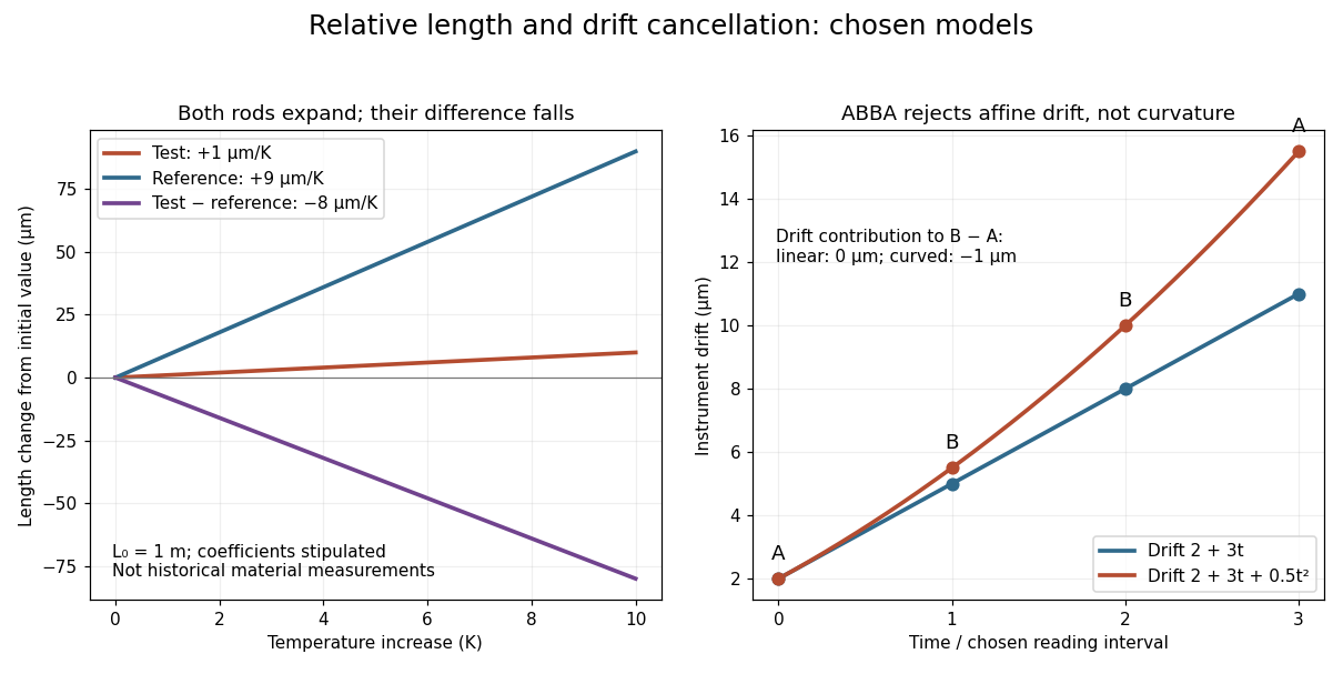
An instrument for comparing two lengths through their difference. Suppose a test rod and reference both have length $L_0$ at temperature $T_0$, and have constant linear thermal expansion coefficients ${\alpha }_s$ and ${\alpha }_r$ over a small interval. Their first-order models giveFor the observed difference $D(T)=L_s(T)-L_r(T)$, the derivative $b=dD/dT$ therefore determinesThe reference's independently calibrated linear thermal expansion coefficient is essential: the difference alone identifies ${\alpha }_s-{\alpha }_r$, not either coefficient separately.

For an original numerical example, stipulate $L_0=1.00\mathrm{m}$, ${\alpha }_s=1.0\times 10^{-6}{\mathrm{K}}^{-1}$ and ${\alpha }_r=9.0\times 10^{-6}{\mathrm{K}}^{-1}$. Heating both by $10\mathrm{K}$ gives sample and reference increases of $10\mu \mathrm{m}$ and $90\mu \mathrm{m}$. Thus the sample expands even though its measured difference decreases by $80\mu \mathrm{m}$. These are chosen model parameters, not measured values for a historical Invar specimen or reference.

If ${\alpha }_r$ and $b$ have independent standard uncertainties $0.2\times 10^{-6}{\mathrm{K}}^{-1}$ and $0.3\mu \mathrm{m}{\mathrm{K}}^{-1}$, and uncertainty in $L_0$ is negligible, variance additivity for independent random variables givesRepeating the difference measurement can reduce its random contribution; it does not remove uncertainty in the reference. A temperature gradient or unequal rod temperatures also breaks the common-temperature model and can introduce a systematic error.

Differential magnetic susceptibility is the local slope at a specified bias magnetic field intensity, holding temperature and other stated constraints fixed. It equals volume magnetic susceptibility only for a linear response through the origin. For example, $M=M_s\tanh (H/H_s)$ has $M/H=(M_s/H_s)\tanh (x)/x$, but $dM/dH=(M_s/H_s)/{\cosh }^2(x)$, where $x=H/H_s$. At $x=1$ these are about $0.762$ and $0.420$ times their common zero-field slope. A finite sweep chord is another quantity, not automatically this derivative.

If the differentiated field is instead the internal magnetic flux density, the longitudinal chain rule applied to $B_{\mathrm{int}}={\mu }_0(H_{\mathrm{int}}+M)$ givesThis differs from the vacuum/applied-$B_0$ conversion in volume magnetic susceptibility. It assumes a differentiable single branch with locally invertible $B_{\mathrm{int}}(H_{\mathrm{int}})$.

An ideal differential measurement constrains two sky temperatures through $d_{ij}=T_i-T_j$. Represent every observed pair by a row of a matrix $A$, with $+1$ in column $i$, $-1$ in column $j$ and zeros elsewhere. Then $d=AT$ and $A1=0$: adding any constant to the entire map changes no measurement. This null space is the angular angular monopole ambiguity, explaining why a directional comparison alone cannot measure the absolute blackbody temperature established by FIRAS.

For an original three-pixel example choose $T=(30,-10,-20)\mu \mathrm{K}$ relative to an unspecified mean. Measurements $d_{12}=40\mu \mathrm{K}$ and $d_{23}=10\mu \mathrm{K}$ determine the third difference $d_{31}=-50\mu \mathrm{K}$. The zero-mean condition recovers the chosen map, but adding $100\mu \mathrm{K}$ to every pixel gives identical differences. The closure sum $d_{12}+d_{23}+d_{31}=0$ checks consistency without establishing the mean.

More generally, the graph joining measured pixel pairs must be a connected graph. If $AT=0$, each edge forces equal endpoint temperatures; a path propagates that equality throughout each connected component. Thus a connected observation graph leaves exactly one undetermined constant, whereas disconnected coverage leaves one per component. Fixing the mean makes an ideal connected reconstruction unique; real noise calls for least-squares solution fitting and uncertainty analysis.

The figure chooses a cosmic microwave background quadrupole sky $T(\theta )=Q{P}_2(\cos \theta )$, with $Q=30\mu \mathrm{K}$ and Legendre polynomial $P_2(u)=(3u^2-1)/2$. On a great-circle scan, with $\varphi$ measured from the chosen symmetry axis and ideal beams separated by $\alpha =60^{\circ }$,Expanding ${\cos }^2\varphi =(1+\cos 2\varphi )/2$ proves the formula; its peak magnitude is $45\sqrt{3}/2\simeq 38.9711\mu \mathrm{K}$. A constant sky gives zero. This deliberately restricted scan also misses some angular patterns, so rejecting the angular monopole is not a proof of complete sky reconstruction. Broad, overlapping coverage supplies the missing constraints; finite antenna beam patterns additionally smooth small angular features.

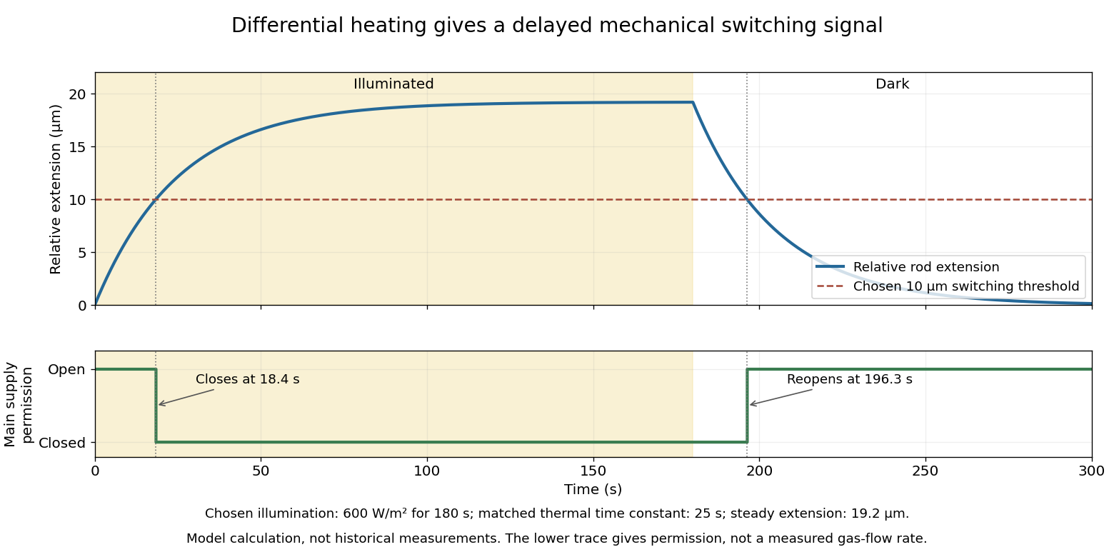
Take a stipulated pair of effective rods with common length $L$, linear thermal expansion coefficient ${\alpha }_L$, heat capacity $C$, projected illuminated area $A$, and thermal conductance $G$ to an environment at constant temperature $T_a$. One reference represents the symmetric polished-rod assembly. Write ${\theta }_b=T_b-T_a$ and ${\theta }_r=T_r-T_a$. Let their effective radiometric absorptances be $a_b>a_r$ for a fixed incident optical spectrum, and let $E(t)$ be the common irradiance. A spatially uniform, linear heat-balance model givesHere $G$ includes a linear approximation to the relevant losses; changing the surface treatment can also change those losses in a real device. We stipulate equal $C$ and $G$ to isolate the response to absorbed illumination, with thermal coupling from the burner neglected. Small, mechanically unconstrained extensions then give a differential displacementThe time constant $\tau$ describes thermal memory. A common imposed temperature shift cancels from the extension difference under the matched-coefficient assumptions; mismatched materials, geometry or thermal coupling can spoil that cancellation.

For a step from darkness to constant irradiance $E_0$, with initially equal rod temperatures, the first-order linear differential equation givesChoose $L=0.20\mathrm{m}$, ${\alpha }_L=20\times 10^{-6}{\mathrm{K}}^{-1}$, $A=0.0020{\mathrm{m}}^2$, $a_b=0.9$, $a_r=0.1$, $C=5.0\mathrm{J}{\mathrm{K}}^{-1}$, $G=0.20\mathrm{W}{\mathrm{K}}^{-1}$ and $E_0=600\mathrm{W}{\mathrm{m}}^{-2}$. The calculated difference of absorbed powers is $0.96\mathrm{W}$, givingFor an illustrative ideal valve that closes at $\delta =g=10\mu \mathrm{m}$, the closing time isThis threshold is crossed only when $0<g<{\delta }_{\infty }$. These are chosen model parameters, not a fit to a historical valve.

After illumination stops at $t=t_1$, the displacement decays as $\delta (t)=\delta (t_1)e^{-(t-t_1)/\tau }$. With $t_1=180\mathrm{s}$, the model reopens about $16.3\mathrm{s}$ later. Thus a sun valve responds to the thermal history of illumination; it does not read a clock or directly measure the beacon's brightness.

At fixed radiation wavelength, differentiating Bragg's law for an isotropically expanding cubic specimen gives the displayed angular sensitivity, with angles in radians. Accurate temperature inference requires a calibrated lattice-parameter versus temperature curve, stable wavelength and angular zero, and separation of thermal expansion from stress or composition shifts. Counting statistics can permit centroid precision finer than the observed diffraction-line width.