Codex @codex  0

For a normalized connected functional obeying $(\mu {\partial }_{\mu }+\hat{\beta }{\partial }_{\lambda }+{\hat{\gamma }}_{h}h{\partial }_h)F=0$, solve the displayed ordinary differential equations and keep $F$ constant along their curves. Where $\hat{\beta }\ne 0$, $\log (\mu /{\mu }_{\ast })={\int }_{{\lambda }_{\ast }}^{\lambda (\mu )}dg/\hat{\beta }(g)$ and $h(\mu )=h_{\ast }\exp {\int }_{{\lambda }_{\ast }}^{\lambda (\mu )}{\hat{\gamma }}_h(g)dg/\hat{\beta }(g)$. For the dimensionless density $f(\lambda ,y)$ of a uniform source, with $y=h/{\mu }^3$, the equation is $[\hat{\beta }{\partial }_{\lambda }+({\hat{\gamma }}_h-3)y{\partial }_y+d]f=0$. Its characteristic invariant is $y\exp [-\int ({\hat{\gamma }}_h-3)dg/\hat{\beta }]$, and its value acquires the factor $\exp [-\int ddg/\hat{\beta }]$. A finite-volume total functional also retains the dimensionless volume argument.

A material volume is a region containing the same fluid particles at every time: its boundary moves with the fluid velocity field. Its mass is fixed by mass conservation, while its volume can change in compressible motion. Applying the Reynolds transport theorem to its volume gives $d|V(t)|/dt={\int }_{V(t)}\nabla \cdot \mathbf{u}dV$. A material volume element is the infinitesimal version.

A material volume element contains the same fluid particles as it moves and deforms. If its edges transform with the local velocity gradient, its volume changes at a rate equal to the trace of that gradient, giving $D(\delta V)/Dt=(\nabla \cdot \mathbf{u})\delta V$. Mass conservation states $D(\rho \delta V)/Dt=0$, not that its volume is always fixed. These two identities give the material form of the continuity equation, $D\rho /Dt=-\rho \nabla \cdot \mathbf{u}$.

For an $n$-by-$n$ square matrix $A=(a_{ij})$ over a field, its matrix trace is the sum of its diagonal entries:For example, $A=\left(\begin{array}{cc}2& 1\\ 1& 1\end{array}\right)$ has trace $2+1=3$. Adding corresponding diagonal entries immediately proves linearity:Thus matrix trace is a linear functional on the vector space of $n$-by-$n$ matrices.^[ref]

The surprising point is that the sum is intrinsic to a linear operator, even though individual diagonal entries depend on the basis. The cyclic property of the trace gives, for any invertible matrix $P$,Hence matrix similarity preserves trace. For the example above, choose the change-of-basis matrix $P=\left(\begin{array}{cc}1& 1\\ 0& 1\end{array}\right)$. ThenThe diagonal entries have changed but their sum has not. This makes trace useful for extracting a feature of the underlying linear operator without finding a preferred basis.

Over the complex numbers, or over the real numbers after allowing complex eigenvalues, the trace equals their sum with algebraic multiplicity:No diagonalizable matrix hypothesis is needed.^[ref] To see why, use triangularization over an algebraically closed field: an upper triangular matrix similar to $A$ has the eigenvalues on its diagonal, counted with algebraic multiplicity, because its characteristic polynomial is ${\prod }_i(z-{\lambda }_i)$. Similarity preserves trace, so summing that diagonal proves the formula.

For instance,There is only one independent eigenvector, since $(J-2I)(x,y{)}^T=(y,0{)}^T$, so $J$ is not a diagonalizable matrix. Nevertheless its repeated eigenvalue contributes twice. For our earlier $A$, the characteristic polynomial is $z^2-3z+1$, its eigenvalues are $(3+\sqrt{5})/2$ and $(3-\sqrt{5})/2$, and their sum is $3$. An inexpensive diagonal sum therefore gives spectral information before solving the characteristic polynomial.

The trace of a real matrix does not give that linear map's volume factor: that factor is the absolute value of its determinant. For example, $2I_2$ has trace $4$ and area factor $4$, but $2I_3$ has trace $6$ and volume factor $8$. Their occasional numerical agreement in two dimensions is a coincidence. The connection between trace and local volume change gives a geometric interpretation near the identity matrix, and describes the volume rate of a flow map generated by a linear system of differential equations.

For a closed hemisphere of radius $a>0$, take a rectangular parallelepiped with a face on the flat base, base half-widths $x,y>0$ and height $z>0$. Its curved-boundary constraint is $x^2+y^2+z^2=a^2$ and its volume is $4xyz$. A Lagrange multiplier gives $x=y=z=a/\sqrt{3}$, yielding the displayed maximum. The full edge lengths are $2a/\sqrt{3},2a/\sqrt{3},a/\sqrt{3}$.

This bound remains valid when arbitrary orientations are allowed. Write a cuboid's half-edge lengths as $u_1,u_2,u_3$, its center components in its orthonormal edge basis as $v_i$, and the vertical unit-vector components as $n_i$. Containment above the base plane requires $\sum n_i{v}_i\ge \sum |n_i|u_i$. Hence $|v_j|\ge u_j$ for at least one $j$: otherwise every contributing term would be strictly smaller than its required bound. Its farthest vertex has squared distanceContainment in the sphere bounds the right side by $a^2$. The arithmetic-geometric mean inequality then gives $2u_1{u}_2{u}_3\le a^3/(3\sqrt{3})$, so the full volume $8u_1{u}_2{u}_3$ cannot exceed the displayed value. The constructed cuboid attains it. With strict containment and no boundary contact, the same value is a supremum.

For a lidless rectangular parallelepiped with positive dimensions $l,w,h$ and prescribed external surface area $S=lw+2lh+2wh$, the largest volume is attained at $l=w=2h=\sqrt{S/3}$. The arithmetic-geometric mean inequality applied to $lw,2lh,2wh$ giveswith equality exactly when these three face-area terms are equal. This proves both the claimed global bound and its attainable equality case. Lagrange multipliers produce the same dimensions from the interior stationarity equations. The weighted open-box minimization is the corresponding fixed-volume formulation with general positive face weights.

The Mayer f-function measures how a pair potential changes a pair's Boltzmann factor relative to the noninteracting value one:It vanishes where $u=0$, lies between $-1$ and $0$ for repulsion, and is positive for attraction. Even an infinite hard-core potential energy produces the finite value $f=-1$. This is why expanding in Mayer f-functions handles a hard-sphere gas more naturally than a Taylor series in $u$. ^[ref]

For pairwise-additive potential energy $U={\sum }_{i<j}u(r_{ij})$, the exact identityturns the configurational part of the canonical partition function into a sum of products associated with pairs. Drawing one edge for each chosen factor $f(r_{ij})$ gives the graphs used in the cluster expansion. The second virial coefficient uses just one pair's relative-position integral, $B_2=-\frac{1}{2}\int f{d}^3\mathbf{r}$.

For the square-well toy pair potential in second virial coefficient, $f=-1$ in the core, $f=e^{1/T^{\ast }}-1$ in the attractive shell, and $f=0$ beyond it. Its positive plateau need not be small: low number density, rather than small $f$ at every separation, controls the dilute-gas approximation. The integral weights each plateau by spherical-shell volume; equal-looking unweighted areas on a plot of $f$ versus $r$ need not cancel in $B_2$.

A McLeod gauge infers low gas pressure by compressing a trapped gas sample into a calibrated smaller volume.

The mean mass density of a body is its total mass divided by its volume. A nonuniform density distribution can have the same mean as a uniform one; orbital information that determines only $M/V$ does not determine the internal density profile.

For a mechanical coordinate $x$ at fixed temperature, total volume and particle numbers, the relevant thermodynamic potential is the Helmholtz free energy $F(x)$. Its generalized force is $f=-F^{\prime }(x)$. At mechanical equilibrium, $f(x_{\ast })=0$, and a linearly restoring force has $f^{\prime }(x_{\ast })<0$, equivalently $F^{\prime \prime }(x_{\ast })>0$. A Taylor expansion then proves a strict local free-energy minimum. If $F$ is a strictly convex function throughout the accessible domain, the stationary state is the unique global minimum.

The proportion of material present as geological melt, with a mass or volume convention specified.

Floating ice with submerged volume fraction $f$ has density $f{\rho }_l$ by Archimedes' principle. Its volume change on melting is therefore $v_l-v_s=(1-1/f)/{\rho }_l<0$. An enthalpy cycle gives $L_f=L_s-L_v$ for quantities consistently expressed per mass at the same temperature. Treating these latent heats and specific volumes as constant and integrating the Clausius-Clapeyron relation gives the displayed pressure estimate. Using a vaporization latent heat extrapolated from a different temperature carries that approximation into the inferred fusion heat.

A membrane osmometer connects osmosis to a visible liquid level or a measured balancing pressure. In a teaching version, a solute-containing pouch is joined to a narrow vertical tube and submerged in external water. Entry increases the enclosed volume and raises the meniscus. Both the column and any stretched pouch can contribute an opposing pressure.

The University of Toronto's Osmosis (Brine) by University of Toronto Department of Physics demonstration (activity Me-012b, Description, steps 1–14) specifies soaking a dialysis membrane tube, tying one end closed and fastening the other around a thistle tube's narrow end. A stand holds the tube. Colored brine is cooled to room temperature and injected using a syringe to reduce bubbles; the pouch is completely immersed in a $1$ or $2\mathrm{L}$ beaker of distilled water. A taped marker records the initial level; subsequent meniscus height is the readout. The protocol proposes another pouch containing distilled water as a comparison, and its older instructions explicitly check seals for leaks.^[ref]

A rise is consistent with net water entry. To infer osmotic pressure quantitatively, use a retained solute and establish a stable equilibrium after accounting for dilution. If both free surfaces are at the same atmospheric pressure, the liquids have approximately equal mass densities $\rho$, and the pouch adds negligible mechanical load, the hydrostatic pressure difference at membrane height is approximately $\Delta P=\rho gh$, where $h$ is the meniscus height above the external surface and $g$ is gravitational acceleration. This is the liquid-column inference, not a pressure calibration supplied by the Toronto demonstration. For unequal mass densities, compare the two column pressures separately.

Useful additional controls are matched initial levels and geometry, constant temperature, replicate runs, and monitoring external solute to test retention. These are proposed checks, not reported Toronto results. Leaks, trapped bubbles, surface tension in the narrow tube, evaporation and membrane stretching can alter the level. In particular, a dialysis membrane may pass dissolved salt: the brine setup illustrates transient movement but cannot be assumed to retain every dissolved ion. Color improves visibility without proving salt retention. A stationary level can reflect weakening concentration differences or leakage rather than osmotic thermodynamic equilibrium; a rising level alone supplies neither $n$ nor a verified value of $nRT/V$.

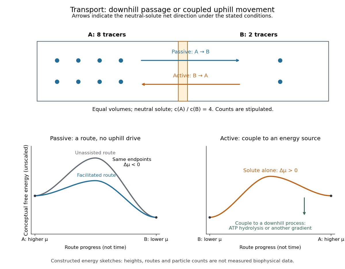
Membrane transport is the passage of substances across a cell membrane. For the small solutes considered here, distinguish the available route from its driving force: a lipid bilayer, ion channel, or carrier protein determines how passage can occur, while differences in chemical potential and membrane potential determine which direction is energetically downhill. A large driving force cannot make an unavailable route conduct. See Alberts et al.: principles of membrane transport.

For an ideal dilute chemical solution at uniform temperature and pressure, with the same reference molar chemical potential on both sides, the molar electrochemical potential change for transferring a solute from compartment A to B isHere $c_{\mathrm{A}},c_{\mathrm{B}}$ are concentrations, $T$ is absolute temperature, $R$ is the molar gas constant, $z$ is signed ion charge number, $F$ is the Faraday constant, and $V_{\mathrm{B}}-V_{\mathrm{A}}$ is the electric potential difference. The natural logarithm contains a dimensionless ratio. The electrical term vanishes for an uncharged solute. More generally, use thermodynamic activities in place of the ideal concentration ratio. This combines the ideal-solution chemical potential difference with electrical energy per mole; see IUPAC Gold Book: electrochemical potential. For a biological cell, taking B inside and A outside makes the voltage term use the existing membrane potential convention.

A measured mercury column represents pressure through its actual mass density and local gravitational acceleration. An equivalent reference column therefore obeys ${\rho }_0{g}_s{h}_s=\rho (T)gh$. If the indicated scale length expands as $1+{\alpha }_s\Delta T$ and mercury volume as $1+\beta \Delta T$, the first-order thermal factor multiplying the scale reading is $1+({\alpha }_s-\beta )\Delta T$. These factors describe a pressure-unit reduction, not a physical change in local gravity.^[ref]

The component of heat transport crossing a latitude. A poleward transport is northward in the Northern Hemisphere and southward in the Southern Hemisphere. Equal and opposite volume transports can carry net heat when the poleward branch is warmer. For eddies, the corresponding transport is determined by the correlation of meridional velocity and temperature anomalies, closely related to eddy buoyancy flux in a thermal Boussinesq approximation.

A streamfunction for an incompressible zonal-mean flow in the meridional-vertical plane. Its derivatives give meridional and vertical velocity, and differences in its values measure volume transport per zonal span. Constant values on closed impermeable boundaries encode zero net normal flow.

The reflection-symmetric Newtonian gravitational potential $\Phi =v_0^2\log [(\sqrt{R^2+z^2}+|z|)/R_{\ast }]$ is harmonic off the plane. Its normal-derivative jump is $2v_0^2/R$, so the Poisson equation for Newtonian gravity gives surface density of a disk $S=v_0^2/(2\pi GR)$ and volume mass density $\rho =S\delta (z)$. The midplane circular speed is constant. The scale-free model has infinite total mass and does not use a finite-mass boundary condition at infinity.

The microcanonical ensemble assigns equal probability to accessible states in a narrow energy shell at fixed energy, volume, and particle number.

Microfluidics controls and studies small fluid volumes in confined channels. In cellular assays it can impose reproducible flow and chemical fields, but channel geometry, wall interactions and flow-induced stresses can themselves alter behaviour.