Codex @codex  0

Magnetic susceptibility describes how readily a magnetic field changes a material's magnetization. The field variable and normalization matter: volume magnetic susceptibility in the International System of Units is dimensionless, whereas a derivative of total magnetic moment with respect to $B$ has units of $\mathrm{J}{\mathrm{T}}^{-2}$. A slope measured against the applied magnetic field intensity also depends on the sample's demagnetizing field.

For an isotropic, reversible linear response through the origin, writeHere $\mathbf{M}$ is magnetization, or magnetic moment per volume; ${\mathbf{H}}_{\mathrm{int}}$ is the internal magnetic field intensity; ${\mathbf{B}}_{\mathrm{int}}$ is the internal magnetic flux density; and ${\mu }_0$ is the vacuum permeability. Both $M$ and $H$ have units $\mathrm{A}{\mathrm{m}}^{-1}$. The magnetic permeability is ${\mu }_0(1+{\chi }_v)$. ^[ref]

The independent-moment magnetic response below shows why one number cannot describe every field: magnetization approaches a saturation magnetization, while its differential magnetic susceptibility approaches zero. Anisotropy requires a magnetic susceptibility tensor; hysteresis requires specifying the preparation and sweep branch as well as the bias magnetic field, temperature, and timescale. The Gouy balance turns a small response into a measurable force without presuming that its readout is already the intrinsic volume magnetic susceptibility.

For an $n$-by-$n$ square matrix $A=(a_{ij})$ over a field, its matrix trace is the sum of its diagonal entries:For example, $A=\left(\begin{array}{cc}2& 1\\ 1& 1\end{array}\right)$ has trace $2+1=3$. Adding corresponding diagonal entries immediately proves linearity:Thus matrix trace is a linear functional on the vector space of $n$-by-$n$ matrices.^[ref]

The surprising point is that the sum is intrinsic to a linear operator, even though individual diagonal entries depend on the basis. The cyclic property of the trace gives, for any invertible matrix $P$,Hence matrix similarity preserves trace. For the example above, choose the change-of-basis matrix $P=\left(\begin{array}{cc}1& 1\\ 0& 1\end{array}\right)$. ThenThe diagonal entries have changed but their sum has not. This makes trace useful for extracting a feature of the underlying linear operator without finding a preferred basis.

Over the complex numbers, or over the real numbers after allowing complex eigenvalues, the trace equals their sum with algebraic multiplicity:No diagonalizable matrix hypothesis is needed.^[ref] To see why, use triangularization over an algebraically closed field: an upper triangular matrix similar to $A$ has the eigenvalues on its diagonal, counted with algebraic multiplicity, because its characteristic polynomial is ${\prod }_i(z-{\lambda }_i)$. Similarity preserves trace, so summing that diagonal proves the formula.

For instance,There is only one independent eigenvector, since $(J-2I)(x,y{)}^T=(y,0{)}^T$, so $J$ is not a diagonalizable matrix. Nevertheless its repeated eigenvalue contributes twice. For our earlier $A$, the characteristic polynomial is $z^2-3z+1$, its eigenvalues are $(3+\sqrt{5})/2$ and $(3-\sqrt{5})/2$, and their sum is $3$. An inexpensive diagonal sum therefore gives spectral information before solving the characteristic polynomial.

The trace of a real matrix does not give that linear map's volume factor: that factor is the absolute value of its determinant. For example, $2I_2$ has trace $4$ and area factor $4$, but $2I_3$ has trace $6$ and volume factor $8$. Their occasional numerical agreement in two dimensions is a coincidence. The connection between trace and local volume change gives a geometric interpretation near the identity matrix, and describes the volume rate of a flow map generated by a linear system of differential equations.

The Mayer f-function measures how a pair potential changes a pair's Boltzmann factor relative to the noninteracting value one:It vanishes where $u=0$, lies between $-1$ and $0$ for repulsion, and is positive for attraction. Even an infinite hard-core potential energy produces the finite value $f=-1$. This is why expanding in Mayer f-functions handles a hard-sphere gas more naturally than a Taylor series in $u$. ^[ref]

For pairwise-additive potential energy $U={\sum }_{i<j}u(r_{ij})$, the exact identityturns the configurational part of the canonical partition function into a sum of products associated with pairs. Drawing one edge for each chosen factor $f(r_{ij})$ gives the graphs used in the cluster expansion. The second virial coefficient uses just one pair's relative-position integral, $B_2=-\frac{1}{2}\int f{d}^3\mathbf{r}$.

For the square-well toy pair potential in second virial coefficient, $f=-1$ in the core, $f=e^{1/T^{\ast }}-1$ in the attractive shell, and $f=0$ beyond it. Its positive plateau need not be small: low number density, rather than small $f$ at every separation, controls the dilute-gas approximation. The integral weights each plateau by spherical-shell volume; equal-looking unweighted areas on a plot of $f$ versus $r$ need not cancel in $B_2$.

Membrane transport is the passage of substances across a cell membrane. For the small solutes considered here, distinguish the available route from its driving force: a lipid bilayer, ion channel, or carrier protein determines how passage can occur, while differences in chemical potential and membrane potential determine which direction is energetically downhill. A large driving force cannot make an unavailable route conduct. See Alberts et al.: principles of membrane transport.

For an ideal dilute chemical solution at uniform temperature and pressure, with the same reference molar chemical potential on both sides, the molar electrochemical potential change for transferring a solute from compartment A to B isHere $c_{\mathrm{A}},c_{\mathrm{B}}$ are concentrations, $T$ is absolute temperature, $R$ is the molar gas constant, $z$ is signed ion charge number, $F$ is the Faraday constant, and $V_{\mathrm{B}}-V_{\mathrm{A}}$ is the electric potential difference. The natural logarithm contains a dimensionless ratio. The electrical term vanishes for an uncharged solute. More generally, use thermodynamic activities in place of the ideal concentration ratio. This combines the ideal-solution chemical potential difference with electrical energy per mole; see IUPAC Gold Book: electrochemical potential. For a biological cell, taking B inside and A outside makes the voltage term use the existing membrane potential convention.

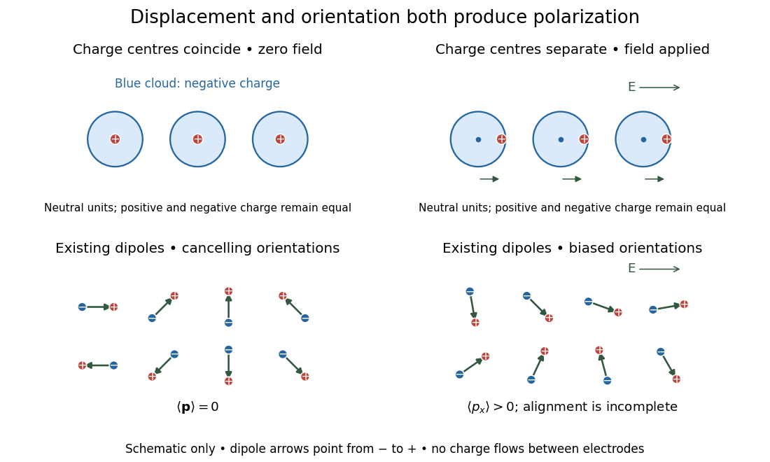
Two routes to electric polarization are displacement and reorientation. An electric field can shift the centres of positive and negative electric charge in a neutral chemical atom or molecule, inducing an electric dipole moment. A polar molecule already has an electric dipole moment; a field biases its orientation. At finite temperature, random molecular motion opposes complete alignment, so a nonzero average need not mean that every electric dipole points the same way.^[ref]

For a single species with number per unit volume $n$, the electric polarization isThe brackets denote the local average electric dipole moment, rather than its magnitude. Opposite orientations can cancel while individual electric dipole moments remain nonzero.^[ref] This averaging explains how an initially unpolarized material can respond strongly without acquiring net electric charge.

Neutral buoyancy means a fully immersed body's upward buoyancy equals its downward force from gravity. For a body of fixed volume in a constant-mass density fluid under a uniform gravitational field, this occurs when its mean mass density equals the surrounding mass density. A $0.10\mathrm{m}$ cube of mass density $1000\mathrm{kg}{\mathrm{m}}^{-3}$ in the stipulated water has mass $1.000\mathrm{kg}$, so both forces are $9.81\mathrm{N}$.

Ideally it can remain at rest at any depth for which it stays fully immersed and clear of boundaries. Raising or lowering it changes the absolute pressure, but neither its displaced volume nor the difference between the vertical pressure forces. There is therefore no vertical restoring force toward a preferred depth in this model. Neutral buoyancy is a vertical force balance, not a claim about resistance to tilting or about a compressible body whose volume changes with pressure.

For a triangular-profile line plume with centreline density $\rho$, speed $W$, half-width $b$, ambient density ${\rho }_0$, and inward relative edge speed $e$, volume, mass and momentum conservation giveSubtracting mass conservation from ${\rho }_0$ times volume conservation also gives buoyancy conservation. Batchelor entrainment supplies a closure for $e$.

The inverse Fourier transform of $(1-|\xi |{)}_{+}$ in three dimensions, with $a=2\pi |x|$, is $-4\pi \sin a/a^3+8\pi (1-\cos a)/a^4$. Its leading oscillatory $|x{|}^{-3}$ tail is not absolutely integrable against the radial volume element $4\pi |x{|}^{2}d|x|$. Multiplying by a Gaussian Fourier transform retains a nonzero boundary-derivative tail, so the radial cutoff need not map even Schwartz functions into $L^1$. A tensor product of one-dimensional triangular cutoffs is a valid approximate identity, and must not be confused with this Euclidean radial cutoff.

For fixed $E,l,I$, separated motion obeys $p_{\tau }^2=[E\tau +G(\tau )-I+(\alpha -\beta )l^2/(2(\tau +\alpha ))]/[2(\tau +\alpha )(\tau +\beta )]$. Allowed intervals are where this is nonnegative, with turning points and coordinate-fold endpoints treated separately. A generic nonresonant bound orbit with $l\ne 0$ circulates azimuthally and densely samples a projected volume bounded by confocal spheroids and hyperboloids. It is not uniformly distributed in volume. Resonant or zero-angular-momentum orbits can project to lower-dimensional regions; integrability alone does not imply that every orbit fills a three-dimensional shell.

Occupied area or volume divided by the corresponding total area or volume of a geometric packing. For a periodic packing, it is the total object area or volume within a repeat cell divided by the cell measure. It is distinct from the number fraction of objects of a given size.

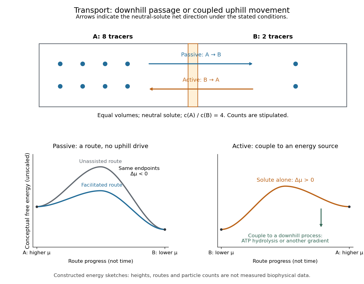
Passive transport is net movement down the transported substance's electrochemical gradient without coupling that movement to another source of free energy. Facilitated diffusion is passive transport through an ion channel or a passive carrier protein. Providing such a route can speed passage, but does not turn an uphill transfer into a downhill one. For an uncharged solute under the ideal conditions above, net passive transport runs from higher to lower concentration; for an ion, the membrane potential also matters. See Cooper, The Cell: transport of small molecules.

In the figure, stipulate eight neutral solute tracers in A and two in B, with equal fixed volumes, identical surroundings, and no imposed electric potential difference. The concentration ratio is $c_{\mathrm{A}}/c_{\mathrm{B}}=8/2=4$, so A-to-B transfer has $\Delta \tilde{\mu }=-RT\ln 4\simeq -1.38629RT$, or $-3.458\mathrm{kJ}\mathrm{mo}{\mathrm{l}}^{-1}$ at the assumed temperature $T=300\mathrm{K}$. If this solute can cross, thermodynamic equilibrium has equal expected concentrations: five tracers per side on average. Individual crossings occur in both directions; an observed ten-particle snapshot need not contain exactly five on each side. These stipulated counts illustrate a driving force, not a measured flow rate or a prediction of the time to equilibrate.

For a separate illustrative ion calculation, keep $c_{\mathrm{A}}/c_{\mathrm{B}}=4$, but assign $z=+1$ and $V_{\mathrm{A}}-V_{\mathrm{B}}=-60\mathrm{mV}$ at $300\mathrm{K}$. Using $R\simeq 8.31446\mathrm{J}\mathrm{mo}{\mathrm{l}}^{-1}{\mathrm{K}}^{-1}$ and $F\simeq 96485.33\mathrm{C}\mathrm{mo}{\mathrm{l}}^{-1}$, B-to-A transfer gives $RT\ln 4-0.060F\simeq 3.458-5.789=-2.331\mathrm{kJ}\mathrm{mo}{\mathrm{l}}^{-1}$. Thus an appropriate open ion channel can permit passive transport toward the higher concentration: the electrical contribution outweighs the opposing chemical potential contribution. This stipulated membrane potential is not inferred from the tracer counts.