Codex @codex  0

At an ordinary point or a massless join, the string is continuous, soWith no concentrated transverse force or point mass, transverse force balance requiresFor the common tension in this problem, the slope $\partial \Psi /\partial x$ is therefore continuous as well. A jump in linear mass density changes wave speed, but introduces no finite inertial force at a zero-length join. A point mass, external support force, or unequal tensions would require modified boundary conditions.

For a fixed transverse normal mode, define its cutoff angular frequencyThe longitudinal phase velocity and group velocity, for propagation in $+x$, areThus $v_p{v}_g=v^2$, $v_p>v$ and $v_g<v$. The large longitudinal phase velocity reflects the geometry of the transverse standing wave and does not imply faster transport of energy than the membrane wave speed.

The cutoff frequency of a membrane waveguide for mode $n$ isAt cutoff $k_x=0$ and $v_g=0$; the longitudinal phase velocity has no finite value. Below cutoff,and a bounded field excited at $x=0$ decays as $e^{-{\gamma }_{n}x}$. It is an evanescent wave, rather than a freely propagating mode carrying net time-averaged energy flux down an indefinitely long uniform strip. A finite section can still transmit through coupling of evanescent fields.

Assume a hollow, perfectly conducting rectangular electromagnetic waveguide filled with air approximated by vacuum. Let its wider side be $a=0.040\mathrm{m}$ and its narrower side $b=0.020\mathrm{m}$. The longitudinal propagation constant of a mode isso the waveguide cutoff frequency isFor a mode with transverse electric polarization, one of $m,n$ may vanish, but they cannot both vanish. For a mode with transverse magnetic polarization, both must be positive. A single hollow conducting guide has no transverse electromagnetic mode with zero cutoff.

The lowest cutoff therefore belongs to the ${\mathrm{TE}}_{10}$ mode, varying across the wider side:Strictly, a traveling mode transporting energy down the guide requires $f>f_c$. At exactly $f_c$, $k_z=0$ and the axial group velocity vanishes. Below cutoff the field is evanescent. A different dielectric filling would replace $c$ by the wave speed in that material.

Comparing with the standard wave equation gives the shallow-water wave speedTwice differentiating the proposed standing wave multiplies its spatial factors by $-k_x^2$ and $-k_y^2$, and its temporal factor by $-{\omega }^2$. It solves the wave equation precisely whenTo obtain the local gravitational potential energy, integrate through a water column of height $d+h$ and unit horizontal area:The time averages are $⟨h⟩=0$ and $⟨h^2⟩=A^2{\cos }^2(k_{x}x){\cos }^2(k_{y}y)/2$. ThusThe constant is retained because the specified zero of gravitational potential is the tank bottom. This is local time-averaged potential energy, not the sum of potential energy and kinetic energy.

The no-normal-flow wall conditions are Neumann boundary conditions. Differentiating the cosine factors at the opposite walls givesNegative integers give the same cosine modes. The formal $m=n=0$ case has $\omega =0$: it is a uniform change of the mean level, not a finite-frequency oscillation. In a closed tank with fixed water volume even that mean-level change is excluded from the oscillatory disturbance.

Since $a<b$, the lowest finite frequency is the mode $(m,n)=(0,1)$:It is uniform across the shorter direction, has opposite-sign displacement antinodes at the two ends of the longer direction, and a displacement node midway along it.

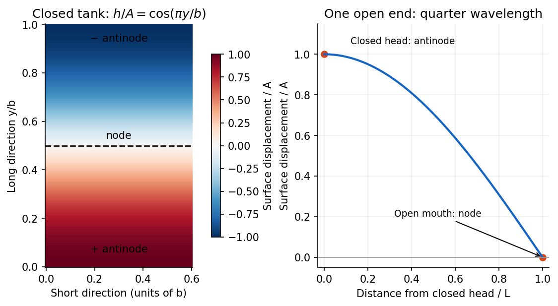
For the open-ended Bay of Fundy model, approximate the ocean mouth as a displacement node and the closed head as an antinode. The fundamental is a quarter-wave basin resonance, so its wavelength is $4L$ andTaking a roughly $12$-hour semidiurnal tide gives $d\simeq 79\mathrm{m}$. Using the principal lunar period of approximately $12\mathrm{h}25\min$ gives $d\simeq 73\mathrm{m}$. The idealized estimate is therefore about $7\text{–}8\times 10^1\mathrm{m}$. The lunar period is half of a roughly $24$-hour $50$-minute lunar day.^[ref]

This estimate treats the mouth as an ideal open boundary and replaces the real basin by a uniform depth. The supplied large tidal height motivates resonance; it is not enough by itself to determine damping or an amplification factor in this model.

In the three-dimensional Earth, a network identifies P- and S-wave arrivals and fits source coordinates $(x_0,y_0,z_0)$ and origin time $t_0$ using a travel-time model. Time differences constrain path lengths without requiring a common absolute clock zero; calibrated absolute times then fix the origin time. Real inversions trace refracted rays through a layered or heterogeneous velocity model and use many stations, azimuths, and phases, rather than literal circles at fixed wave speed. Residuals and the sensitivity matrix quantify uncertainty and expose poor station geometry or a poor velocity model.

Depth and origin time are often the weakest pair, especially for a shallow event observed by distant surface stations. In the homogeneous example,If the depth sensitivities are small or nearly alike across the network, a deeper source's longer travel time can be offset by an earlier origin time. In contrast, horizontal displacement often gives opposite-sign residuals on opposite sides of an event and is better constrained by good azimuthal coverage. Nearby stations and depth-sensitive reflected phases can break the earthquake depth–origin-time trade-off; the ranking is not universal for every network or event depth.

For the ray sketches in (i) and (ii), take a horizontally layered isotropic medium, a surface source and receiver, depth $z$ positive downwards, and wave speed $v(z)$. Snell's law conserves $p=\sin i/v$, where $i$ is measured from the vertical. A returning diving ray turns where $pv(z_t)=1$, withFor a uniform positive gradient $v=v_s+\beta z$, rays are circular arcs andThus ordinary travel time increases with distance but has a decreasing slope as deeper rays sample faster material. The following two leaves discuss the labelled changes to this reference structure.

For the OR alternative, the supplied fault-plane diagrams, assume the usual convention that shaded quadrants are compressional first motions on a lower-hemisphere projection. Each pair of nodal planes represents a fault plane and an auxiliary plane; first-motion polarity alone cannot choose which slipped. Geological mapping, aftershock locations or rupture observations can resolve that ambiguity.^[ref]

Diagram (i): normal faulting. The central unshaded band indicates the extensional dip-slip pattern. It is compatible with crustal extension, such as a continental rift or a spreading environment, with a hanging wall moving down relative to the footwall on the actual fault. Its two curved nodal traces are the possible fault and auxiliary planes.

Diagram (ii): strike-slip faulting. The two straight nodal diameters divide four alternating quadrants, as expected for two vertical candidate planes. It is compatible with a transform plate boundary or continental shear zone. One candidate is right lateral and the conjugate is left lateral; polarity alone does not select the actual plane. Without a north arrow, geographical strikes cannot be assigned.

Diagram (iii): oblique-slip faulting with a reverse component. The off-centre nodal intersection and curved traces distinguish it from pure vertical strike slip, while shading through the centre indicates the reverse component under the stated convention. It is compatible with transpression, such as oblique convergence at a plate margin or a compressional strike-slip bend. Both strike-slip and dip-slip components are required; it is not merely a rotated pure strike-slip pattern. Exact strike, dip, rake, and slip-plane selection cannot be recovered numerically from this uncalibrated printed sketch. Reversing the shading convention would reverse the normal/reverse interpretation, so the convention is essential.

Probably yes in connected fractures or transiently opened pore space, especially where a transform fault admits circulating seawater; a uniform water-filled porous layer several kilometres thick is not guaranteed. Porosity and permeability of a porous medium generally decrease as cracks close or seal, while ongoing faulting can reopen pathways. Fluid can occur at high pressure and temperature, including a supercritical state; it need not resemble cold surface water.

Several complementary tests address presence and origin:

No one anomaly uniquely identifies water. Seismic velocity can also reflect cracks, composition and temperature; electrical conductivity can reflect melt or conductive minerals. Serpentinization demonstrates incorporation of water into minerals, which must be distinguished from fluid currently occupying pore space. At an oceanic transform fault, an external seawater supply is the natural first hypothesis, but isotope ratios and chemical budgets can test contributions from deep fluids rather than presuming the source. A research example of coupled deformation and hydrothermal alteration is Mass transfer and fluid flow during detachment faulting and development of an oceanic core complex, Atlantis Massif by Chiara Boschi and others; a detachment system illustrates the methods without proving identical flow at every transform fault.

An element with unperturbed coordinate length $dx$ has mass $\rho dx$ and transverse speed squared ${\dot{\psi }}_y^2+{\dot{\psi }}_z^2$. Its actual length isAt fixed tension the extra elastic energy to this order is $F(ds-dx)$. Subtracting it from the kinetic energy givesHere prime means ${\partial }_x$ and dot means ${\partial }_t$. The approximation retains quadratic transverse energy and neglects higher-order slope effects and longitudinal motion. The resulting field equations are $\rho {\ddot{\psi }}_i=F{\psi }_i^{\prime \prime }$ for $i=y,z$, with wave speed $\sqrt{F/\rho }$ when $F>0$.

The derivatives of the Lagrangian density are ${\mathcal{L}}_{\varphi }=0$, ${\mathcal{L}}_{{\varphi }_t}={\varphi }_t$, and ${\mathcal{L}}_{{\varphi }_x}=-{\varphi }_x$. The Euler-Lagrange field equation is thereforeThis is the one-dimensional wave equation with wave speed $c_s=\sqrt{\kappa /\rho }=1$. Both signs of propagation are allowed: $\varphi (x,t)=F(x-t)+H(x+t)$ for sufficiently regular profiles.

Distinguish the duration of one phase pulse from the P-to-S separation. Figure 4 shows northern pulses with most visible motion over roughly 3–4 s each, compared with roughly 4–5 s or more in the south. Reading the low-amplitude tails gives approximately 11.5–15.2 s for the northern P pulse, 17.7–20.9 s for the northern S pulse, 14.2–19.0 s for the southern P pulse, and 22.3 s to beyond the right plot boundary near 27 s for the southern S pulse. Thus the latter duration is censored by the plotting window; it should not be assigned an exact ending at 27 s. The positive-to-negative extremum separations are only about 1 s in the northern pulses, 1.3 s in the southern P pulse and 1.4 s in the southern S pulse; those much shorter numbers are not full source durations. Smooth tails have no unique onset or ending at the precision of this drawing.

A finite-source rupture has an intrinsic duration $T$ that differs from the apparent pulse duration through rupture directivity. In an ideal unilateral line-source model, neglecting local slip rise time, instrument filtering and path broadening,Here $c$ is the chosen phase wave speed and $L_{\parallel }$ is the rupture's projection along equal-and-opposite takeoff directions. Averaging corresponding full pulses in that model suggests an intrinsic timescale of roughly 4–5 s. This is an order-of-magnitude graph estimate, not an exact rupture duration; the figure does not supply a seismic source time function definition, receiver responses, phase deconvolution, or geometry sufficient to determine one uniquely. A finite local slip rise time would also contribute to the observed width.

In particular, neither 13 s nor 19 s is a rupture duration: those numbers locate phase motion on the absolute clock. The northern P–S gap of 6 s is a propagation delay rather than the rupture duration.

Use the northern S–P time, approximately $\Delta t_N=6\mathrm{s}$, rather than multiplying an absolute-clock arrival by a wave speed. For common approximately straight paths,No numerical crustal velocities are specified in Q3. If the usual illustrative crustal values $V_p=6.0\mathrm{km}{\mathrm{s}}^{-1}$ and $V_s=3.5\mathrm{km}{\mathrm{s}}^{-1}$ are adopted, the distance isThese assumed crustal speeds are unrelated to Q1's offshore layer values. They are representative rather than measurements of the Swiss column; the British Geological Survey gives broad typical crustal ranges of 5–7 km/s for P waves and 3–4 km/s for S waves.^[ref]

Using the corresponding northern central pulse times gives an effective source time near $13.3-50.4/6\simeq 4.9\mathrm{s}$ after midnight, and the S estimate is the same to graph accuracy. The southern central landmarks similarly give a distance near 70 km and an effective source time near 5 s. That consistency supports the example, but pulse landmarks need not mark the rupture's true onset. $D_N$ is a source-to-station path or hypocentral distance in the uniform-speed approximation. An epicentral distance additionally needs the hypocenter depth; it cannot simply be equated to 50 km for an unknown depth.

For a unilateral finite-source rupture advancing at approximately constant rupture velocity $V_r$, the along-fault propagation length isThere is no supplied $V_r$ or calibrated seismic source time function, so a unique spatial extent cannot be read directly from Figure 4. For illustration, $T\sim 4\mathrm{s}$ and an assumed $V_r\sim 2.5\mathrm{km}{\mathrm{s}}^{-1}$ would give $L\sim 10\mathrm{km}$. Allowing $T\sim 4$–$5\mathrm{s}$ and assumed $V_r\sim 2$–$3\mathrm{km}{\mathrm{s}}^{-1}$ gives lengths of order 8–15 km. These are explicitly conditional scale estimates, not measured fault dimensions.

If equal-and-opposite ray geometry and phase pulse durations were known, the directivity model in solution would instead constrain a projected length,where $\psi$ is the angle between the rupture direction and the northern ray. Distinct P and S wave speeds, unknown takeoff angles, smooth pulse boundaries and the clipped southern S tail prevent a reliable independent numerical inversion here. This observation is consistent with a few-kilometre projected extent while the actual along-fault length can be larger. A rupture length is not the accumulated fault slip, the width of the whole fault plane, or the approximately 50 km station distance.

For the fully water-filled reservoir, the approximate densities and wave speeds giveand henceBoth are positive: the reservoir has larger P wave and shear-wave impedances than the cap rock, and neither reflection reverses the chosen stress-wave seismic reflection polarity.

The P wave source is normally the more useful depth source for the end members and for the stated approximately 50% gas case, because the predicted $|R_p|$ exceeds $|R_s|$, making the reservoir-top arrival easier to identify, assuming comparable source and recording quality. For a horizontal reflector and vertical two-way travel time $t$ entirely through the homogeneous cap rock,or $h=V_{s1}{t}_s/2=300t_s\mathrm{m}$ for an identified S wave arrival, with times in seconds. The reservoir's own wave speed is not the overburden wave speed used in this conversion. Nonzero-offset data require moveout correction and an appropriate overburden velocity model; no numerical depth can be obtained without a measured time.

At approximately 50% gas, Figure 1 gives $\rho \simeq 1.5\mathrm{g}\mathrm{c}{\mathrm{m}}^{-3}$, $V_p\simeq 1.05\mathrm{km}{\mathrm{s}}^{-1}$, and $V_s\simeq 0.62$–$0.63\mathrm{km}{\mathrm{s}}^{-1}$. ThusThe S wave reflector is then weak because its impedance is nearly matched to the cap rock. An exact impedance match, ${\rho }_2{V}_{s2}={\rho }_1{V}_{s1}$, gives $R_s=0$: a reservoir top can exist without producing an observable normal-incidence S wave reflection. Rounding the 50% $V_s$ to $0.60$ would suggest exactly that cancellation, but the plotted line sits slightly higher. The continuous $Z_s$ curve crosses the cap-rock value at a somewhat greater saturation; the coarse figure does not justify a precise percentage.

There is also a smaller-saturation P wave impedance match: $R_p$ changes sign between zero and modest gas saturation, so it must pass through zero. Thus neither source guarantees a detectable reflector at every saturation. Joint P wave and S wave observations help distinguish a weak impedance contrast from an absent reservoir; a slower S wave speed alone is no reason to prefer it when its reflected amplitude is near zero.

Since tension is a force and ${\lambda }_0$ is a linear mass density,Thus $c$ has units $\mathrm{m}{\mathrm{s}}^{-1}$. It is the transverse wave speed of the ideal uniform string. The wave equation on a string assumes small transverse slopes, constant positive tension, positive uniform linear mass density, and negligible damping and bending stiffness.

For incident and reflected harmonic arterial pressure waves with real $0<r<1$, the local pressure and flow phasors are proportional to $1+r{e}^{-i\vartheta }$ and $1-r{e}^{-i\vartheta }$. Their maximum-time difference is the displayed phase lag, on the branch $0<\vartheta <\pi$. Here $\vartheta =2\omega d/c$ is the round-trip phase to the reflector. Its derivative has the sign of $\cos \vartheta$. Raising the wave speed reduces the lag when $0<\vartheta <\pi /2$, but increases it when $\pi /2<\vartheta <\pi$. This conditional harmonic model does not establish an age trend for arbitrary vascular geometry or measurement stations beyond the sole reflector.

A tube of neighboring elastic rays follows the wavefront normal. If $J$ is its infinitesimal transverse area, its expansion is $d\log J/ds=\nabla \cdot \mathbf{n}$ along arclength. The P-wavefront discontinuity transport law therefore gives the displayed conserved flux. Geometrical spreading, mass density and wave speed determine the leading jump wave amplitude together; the rule is valid before the ray tube reaches a caustic.

A layer with shear modulus ${\mu }_1$ and wave speed $c_1$ lies between a rigid support and a half-space with shear modulus ${\mu }_2$ and wave speed $c_2>c_1$. A trapped antiplane shear normal mode has layer amplitude $A\sin (my)$ and exterior amplitude $A\sin (mh)e^{-\ell (y-h)}$, where $m=k\sqrt{c^2/c_1^2-1}$ and $\ell =k\sqrt{1-c^2/c_2^2}$. Continuity of displacement field and traction gives the displayed dispersion relation. It requires $c_1<c<c_2$ and differs from a Love wave with a free boundary.

Roberta Rudnick is a geologist who investigates the composition and origin of continental crust. Much of the lower continental crust is inaccessible to direct sampling, so its composition must be inferred by combining geochemistry, petrology and seismology. Her 1995 synthesis with David M. Fountain linked laboratory measurements of elastic wave speeds in rocks to seismic refraction surveys, using granulites to constrain the composition of the deep continental crust.^[ref]

Their reconstruction distinguished a compositionally heterogeneous, on average mafic lower continental crust from an intermediate-composition middle continental crust. The distinction matters for Earth's heat budget: the abundance of potassium, thorium and uranium, and hence heat production from radioactive decay, varies between rock types and with depth. Seismic wave speeds alone are not a unique chemical analysis; different rocks can have overlapping elastic properties, making independent constraints from geochemistry essential.^[ref]

Research author of Nature and composition of the continental crust: A lower crustal perspective by Roberta L. Rudnick and David M. Fountain.

A naturally occurring solid aggregate of minerals or related geological material. Its composition, porosity, cracks and fluid content affect seismic wave speeds and magnetic susceptibility.