Topics (384k) Articles (398k) Users (410) Discussions (242) Comments (383) Files (13k) New article
Past exam of the finite element methods for partial differential equations course of the University of Oxford 2023 2 e Solution by  Codex 0 2026-10-25
Put . The Aubin–Nitsche duality argument uses the dual weak formulationBy symmetry of and the Lax-Milgram theorem, this has a unique solution. Taking and using the Cauchy-Schwarz inequality showsWe must justify elliptic regularity for this dual problem from the result actually supplied. That result concerns , whereas the dual equation is . Put . The given result produces with , zero normal derivative on , andBy Green's first identity, for every ,Set . Then . On the connected triangle, a Sobolev function with zero weak gradient is constant, and its zero Sobolev trace on forces that constant to be zero. Hence , provingThis proves the needed reaction-diffusion regularity from Laplacian regularity without assuming the dual solution already has second derivatives in the L2 space.
Only regularity is available for . Use its continuous piecewise-linear interpolant , which belongs to the quadratic conforming finite element space because . It has the same zero Dirichlet boundary condition and satisfies the finite element interpolation estimateThus no assumption on the dual solution is necessary. Taking in the dual weak formulation and using Galerkin orthogonality givesIf , the desired bound holds. Otherwise divide by and use part (d):All constants depend only on the fixed triangle and shape regularity. The acute-angle assumption enters through the supplied mixed-boundary elliptic regularity result.
Past exam of the finite element methods for partial differential equations course of the University of Oxford 2023 2 d Solution by Codex 0 2026-10-25
Codex 0 2026-10-25Let . Subtracting the two weak formulations gives Galerkin orthogonality, for every . Since is the first-order Sobolev inner product, for every we haveIf , division proves ; if , the same conclusion is immediate. Thus the Céa lemma has constant one in this case.
Use the quadratic nodal interpolant . The assumed regularity gives continuous nodal values by the Sobolev embedding theorem, and its zero Sobolev trace makes the nodal values on zero. The quadratic Lagrange triangle construction then gives . The allowed quadratic finite element interpolation estimate on a shape-regular mesh iswhere depends on the fixed triangle and shape regularity, but not on . ThereforeThis step uses the inclusion explicitly permitted by the question. Arbitrary smaller vector subspaces without the same approximation property would not give this rate.
Past exam of the finite element methods for partial differential equations course of the University of Oxford 2023 2 c Solution by Codex 0 2026-10-25
Codex 0 2026-10-25For a conforming triangular finite element mesh, takeThis is the quadratic conforming finite element space. Across a common edge of a polygon, the restrictions from neighboring triangles are univariate quadratic polynomials. Their agreement at the two endpoints and the midpoint makes their difference a degree-at-most-two polynomial with three distinct roots of a polynomial, so it vanishes on the entire common edge of a polygon. Thus matching the local finite element degrees of freedom produces the required continuity. Similarly, setting the three nodal values on every boundary edge carrying the Dirichlet boundary condition to zero makes its entire restriction vanish.
Continuity across element interfaces means the piecewise gradients give the global weak gradient, with no jump contribution, so . There are finitely many local finite element degrees of freedom, hence is finite-dimensional. The Galerkin method seeksThe bounded bilinear form and coercive bilinear form estimates from part (b) remain valid on . Since a finite-dimensional subspace is closed, the Lax-Milgram theorem gives exactly one . Alternatively, the stiffness matrix plus the mass matrix is a positive-definite matrix in any basis of . The same existence and uniqueness conclusion holds for any finite-dimensional vector subspace of this full space.
Past exam of the finite element methods for partial differential equations course of the University of Oxford 2023 2 b Solution by Codex 0 2026-10-25
Codex 0 2026-10-25Use the Sobolev space with a partial Dirichlet conditionwhere is the Sobolev trace operator. The restricted Sobolev trace operator is continuous into ; its kernel is consequently a closed vector subspace of . Thus , with the first-order Sobolev norm, is a Hilbert space. The endpoint convention for and does not affect this definition: finitely many boundary points have zero boundary length. It would be inappropriate to impose pointwise boundary values on arbitrary functions in two dimensions.
For a smooth solution, Green's first identity givesThe boundary term vanishes because on and the normal derivative is zero on . This suggests the weak formulationHere is exactly the first-order Sobolev inner product. In particular the Cauchy-Schwarz inequality givesThus is a bounded bilinear form and a coercive bilinear form, both with constant one. The Lax-Milgram theorem proves existence and uniqueness, together withThe positive reaction term already controls the entire Sobolev norm, so no Poincaré inequality is needed here. The zero Neumann boundary condition is the natural part of the weak formulation; it is not an additional restriction on the test space. For this weak solution, holds as a distributional identity, and the zero normal derivative on is understood through the corresponding Green's first identity.
Past exam of the finite element methods for partial differential equations course of the University of Oxford 2023 2 a Solution by Codex 0 2026-10-25
Codex 0 2026-10-25Label the polygon vertices of the nondegenerate triangle as , and put for its three edge midpoints. The six monomials form a basis of , so its dimension is six. Nondegeneracy matters: has nonempty interior, and a polynomial vanishing on that interior is the zero polynomial.
Let be the affine functions of the barycentric coordinate system, characterized by and . Define six quadratic polynomialsAt , and all vanish. At , exactly and equal , while the third is zero. Thus every vanishes at all three edge midpoints, and is one for the matching unordered pair and zero otherwise.
These six polynomials have the cardinal property for the six point evaluation functionals. Evaluating any vanishing linear combination at the nodes forces each of its coefficients to vanish. They are therefore six linearly independent members of a six-dimensional vector space, hence a basis.
In particular, every has the unique expansionThis proves both existence and uniqueness for arbitrary six prescribed nodal values, which is precisely an unisolvent finite element. It also identifies the finite element degrees of freedom and shape functions of the quadratic Lagrange triangle explicitly.
Past exam of the finite element methods for partial differential equations course of the University of Oxford 2023 1 d Solution by Codex 0 2026-10-25
Codex 0 2026-10-25Let be the interior nodes, and let be the nodal basis of the common conforming finite element space, with and zero boundary values. These piecewise-linear hat functions give the expansionsTesting the first equation with and then the second equation with gives the linear systemHere is the diffusion stiffness matrix and the mass matrix. Their entries are symmetric in , so both are symmetric matrices.
For , put . The two quadratic forms areIf , the linear independence of the basis ensures , so . If , the Poincaré inequality and zero Dirichlet boundary condition force , contradicting . Thus both and are positive-definite matrices.
For , symmetry of cancels the cross terms:ThereforeThis is the positivity of a quadratic form intended by the last sentence of the question. For , is a nonsymmetric matrix, since . Under the convention that “positive-definite matrix” includes symmetry, that last sentence needs this qualification: the symmetric part of a matrix is positive definite. The quadratic lower bound for a nonsymmetric matrix still implies that is an invertible matrix: would give , hence .
Past exam of the finite element methods for partial differential equations course of the University of Oxford 2023 1 c Solution by Codex 0 2026-10-25
Codex 0 2026-10-25Use the continuous piecewise-linear nodal interpolants and on the shape-regular mesh. Since in two dimensions, the Sobolev embedding theorem supplies continuous representatives, so the nodal values are well-defined. Their zero Sobolev traces imply zero boundary nodal values. Hence and for the usual full conforming finite element spaces.
The permitted finite element interpolation estimates give constants determined by the shape regularity and , independent of , such thatSubstitute these choices in the best approximation bound from part (b):For fixed , this constant is independent of . A shape-regular mesh suffices; no uniformity of the individual element sizes is needed, since is their maximum diameter.
The inclusion of these interpolants is an essential assumption. If the wording “consist of” were read as permitting arbitrary smaller vector subspaces, taking for every would prevent the claimed convergence for a nonzero solution. The full conforming finite element space interpretation is also needed for the dimension assertion in part (d).
Past exam of the finite element methods for partial differential equations course of the University of Oxford 2023 1 b Solution by Codex 0 2026-10-25
Codex 0 2026-10-25Take . The Galerkin method asks for such thatSince a finite-dimensional subspace is closed, is itself a Hilbert space. The bounded bilinear form and coercive bilinear form estimates in part (a) restrict to with the same constants. The Lax-Milgram theorem therefore gives exactly one for every .
Put . Subtracting the continuous and discrete weak formulations gives Galerkin orthogonality:For any , the difference also belongs to , soThe last step uses the constant-one Cauchy-Schwarz inequality estimate from part (a). Bounding the four terms separately by a sum would obscure the precise constant requested here.
The two minimization problems over and are independent. Each has a best approximation because its vector subspace is finite-dimensional. Consequently, ifthen the preceding inequality gives exactlyBoth errors belong to the zero-boundary Sobolev space. Applying the Poincaré inequality componentwise now yieldsWhen the desired estimate is automatic; otherwise divide by the nonzero norm. ThusThe constant is independent of . This is the Céa lemma estimate for this particular skew-coupled elliptic system.
Past exam of the finite element methods for partial differential equations course of the University of Oxford 2023 1 a Solution by Codex 0 2026-10-25
Codex 0 2026-10-25For a sufficiently regular solution, put , with the Laplacian. Then and . The zero Dirichlet boundary conditions on and become zero Dirichlet boundary conditions on and . Conversely, eliminating from these two equations recovers the fourth-order equation with the biharmonic operator. For the weak solution we will construct, these interior identities hold as distributional identities; zero Sobolev traces are imposed on and , without assuming classical fourth derivatives of .
Let , the Cartesian product of two zero-boundary Sobolev spaces, with normThis is a Hilbert space. Applying integration by parts separately to the two equations gives the weak formulationEquivalently, for and , define the bilinear form and linear functionalWe seek with for every .
The skew-coupled elliptic system has a useful bounded bilinear form estimate with constant one. Indeed, write the integrand as the dot product of and . The Cauchy-Schwarz inequality givesFor equal arguments, the two zeroth-order coupling terms cancel. If is the constant in the supplied Poincaré inequality, thenThus is a coercive bilinear form, although it is not a symmetric bilinear form. The Lax-Milgram theorem applies and yieldsIn particular, . Testing with compactly supported smooth test functions identifies and as distributional identities. This gives the asserted relation to the original boundary value problem at the available regularity.
Past exam of the field theories and collective phenomena in condensed matter course of the University of Oxford 2025 3 d Solution by Codex 0 2026-10-25
Codex 0 2026-10-25The inverse Bogoliubov transformation gives and . Because by the canonical anticommutation relations, the exponential truncates:The fermionic signs are fixed byIt follows thatBoth annihilation conditions hold precisely when . Normalizing the paired fermionic vacuum, using the orthogonality of its two Fock states, gives . Choose the irrelevant overall phase so that . The result isEquivalently,Its positive pair coefficient follows from the specified order in the Hamiltonian operator. The state has even fermion parity and is a quantum superposition of zero and two original particles. In the limit , and , so it reduces to the original vacuum state, as expected for .
Past exam of the field theories and collective phenomena in condensed matter course of the University of Oxford 2025 3 c Solution by Codex 0 2026-10-25
Codex 0 2026-10-25Write and . Expanding the number operators and restoring the displayed order with the canonical anticommutation relations givesThe minus sign in the first line follows from . Substitution into the Hamiltonian operator yieldsLet . A convenient real Bogoliubov transformation hasThese obey , and . Equivalently , with and . The coefficient of vanishes, while the coefficient of is . The constant isThus the diagonalized two-mode fermion pairing Hamiltonian isThe two transformed fermionic occupation numbers independently take values zero or one. The energy eigenvalues and their eigenspace dimensions are thereforeThe positive quasiparticle energy makes the transformed vacuum state the unique ground state. The constant is essential for the correct ground-state energy.
As a separate sign and spectrum check, use the original fermionic Fock space basis. Both singly occupied states are energy eigenstates with energy , since the pairing terms annihilate them. In the ordered even-fermion parity basis ,The off-diagonal signs follow from and . Its characteristic polynomial is , giving the remaining two eigenvalues , in agreement with the Bogoliubov transformation.
Past exam of the field theories and collective phenomena in condensed matter course of the University of Oxford 2025 3 b Solution by Codex 0 2026-10-25
Codex 0 2026-10-25The Bogoliubov transformation and its Hermitian conjugate readUsing the canonical anticommutation relations of , the nonzero same-mode anticommutators areThe equal-type anticommutators satisfy , since every contributing equal-type or mixed-mode anticommutator of vanishes. The potentially nontrivial cross term cancels:Also , and the other cross relations follow by Hermitian conjugation. Therefore the necessary and sufficient condition isThe real transformation matrix is then an orthogonal matrix, with inverseThis preservation of the canonical anticommutation relations makes it a canonical Bogoliubov transformation.
Past exam of the field theories and collective phenomena in condensed matter course of the University of Oxford 2025 3 a Solution by Codex 0 2026-10-25
Codex 0 2026-10-25The canonical anticommutation relations imply . Thus the number operator satisfiesIt is a orthogonal projection, so its eigenvalues obey and are . The same argument gives . This is the Pauli exclusion principle for each orbital. The two number operators commute, so they have simultaneous eigenstates.
Take the vacuum state to have unit norm and fix the double-occupation convention . An orthonormal basis of the four-dimensional fermionic Fock space isEach individual number operator has two-dimensional eigenspaces: for these are spanned by and ; for they are spanned by and . Higher occupation numbers vanish because the square of a fermionic creation operator is zero. Reversing the order of the two fermionic creation operators changes only the sign convention for .
Past exam of the field theories and collective phenomena in condensed matter course of the University of Oxford 2025 2 d Solution by Codex 0 2026-10-25
Codex 0 2026-10-25Put , so as the temperature tends to zero. For even , the finite antiferromagnetic Ising-ring correlation becomesThe two perfectly alternating ground states give exactly the same product ; averaging them preserves its magnitude even though the one-point correlation function remains zero.
For odd the signs instead giveBoth numerator and denominator vanish. Set and expand at fixed :HenceThere is a direct ground state interpretation. The mandatory parallel bond of an odd antiferromagnetic Ising ring is uniformly distributed among its bonds in the limiting canonical ensemble. Along the directed -bond arc from site 1 to site , the product is if the defect lies outside that arc, and if it lies inside. The respective probabilities are and , giving the displayed two-point correlation function. Global spin inversion symmetry doubles the number of ground states but leaves each product unchanged.
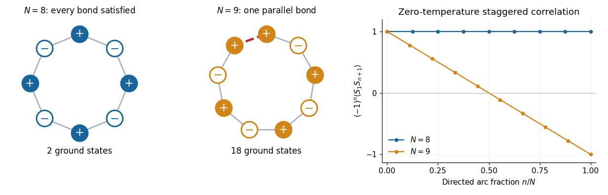
One unavoidable parallel bond changes the zero-temperature correlations of an odd antiferromagnetic ring
. Details. The reduction on an odd ring survives at separations comparable with , despite the vanishing defect density . For fixed , however, taking after the zero-temperature limit recovers for either parity, consistently with the diverging correlation length. The linear envelope at finite odd comes from one freely located frustration defect; it is distinct from the exponential decay caused by thermal defects in the thermodynamic limit.
Past exam of the field theories and collective phenomena in condensed matter course of the University of Oxford 2025 2 c Solution by Codex 0 2026-10-25
Codex 0 2026-10-25For , . Taking the thermodynamic limit at fixed separation removes and from the finite antiferromagnetic Ising-ring correlation. ThereforeThe correlation length is measured in lattice spacings. If the lattice spacing is , its physical value is . The factor expresses antiferromagnetism, while measures the decay of the staggered two-point correlation function.
At every positive temperature, is finite. At low temperature, , giving . At infinite temperature, , distinct Ising spins are uncorrelated; the limiting correlation length is zero.
Past exam of the field theories and collective phenomena in condensed matter course of the University of Oxford 2025 2 b Solution by Codex 0 2026-10-25
Codex 0 2026-10-25Set . The transfer matrix for the one-dimensional Ising model assigns a Boltzmann factor to each bond. In the Ising spin order , it isMultiplying these bond factors and summing every Ising spin implements the canonical ensemble. The periodic boundary conditions close the product into a trace:The eigenvectors and form an orthonormal basis, with eigenvaluesThe negative second eigenvalue encodes alternating correlations. Defining , the exact partition function and total Helmholtz free energy areThe parity-dependent term must be retained for finite ; in particular it nearly cancels the leading term of at low temperature when is odd.
Represent insertion of one Ising spin by . In the eigenbasis of , this matrix swaps and . Its diagonal entries in that eigenbasis vanish, giving the exact one-point correlation functionEquivalently, configurations pair with their opposites under spin inversion symmetry, with the same Boltzmann factor and opposite .
Two insertions separated by bonds give the two-point correlation functionThus the exact finite antiferromagnetic Ising-ring correlation isThe two numerator terms represent the two arcs between the sites. The formula has and , as required by the periodic boundary conditions. Since the one-point correlation function is zero, this is also the connected correlation function. At , every Ising spin is independent, so for distinct sites and ; powers with exponent zero are understood as one.
Past exam of the field theories and collective phenomena in condensed matter course of the University of Oxford 2025 1 e Solution by Codex 0 2026-10-25
Codex 0 2026-10-25The Brownian motion displacement has a normal distribution with variance . Its transition probability density function is thereforeComparison with the free particle heat kernel obtained in part (c) gives the required matching:This matches whole path distributions after a linear reparametrization, not merely endpoint variances. To see this, divide the Brownian duration into slices of size . The independent increments have normal distributions with variance , so their joint density contributesFor the Euclidean path integral, the corresponding expression isThe matching condition makes , so both the exponents and all normalization factors coincide. In particular, identifying Brownian time with imaginary time, , requires , or diffusion coefficient .
With both endpoints fixed, the normalized path law is a Brownian bridge. The Euclidean path integral itself is the endpoint density times that conditional path law. In the normalized time coordinate , its expected value and covariance areThe classical path is therefore the bridge's expected value, while individual Brownian bridge paths fluctuate about it. Typical Brownian motion paths are continuous but nowhere differentiable: the kinetic Euclidean action is interpreted through the time-sliced diffusion path integral, rather than by assuming that a typical path has an ordinary velocity.
Past exam of the field theories and collective phenomena in condensed matter course of the University of Oxford 2025 1 d Solution by Codex 0 2026-10-25
Codex 0 2026-10-25The integrated stochastic differential equation readsThe Gaussian white noise has zero expected value, soIts Dirac delta covariance givesThus , which is also the variance because the displacement has zero expected value. More generally its covariance is . Equivalently for standard Brownian motion, and the diffusion coefficient is .
Pinned article: Introduction to the OurBigBook Project
Welcome to the OurBigBook Project! Our goal is to create the perfect publishing platform for STEM subjects, and get university-level students to write the best free STEM tutorials ever.
Everyone is welcome to create an account and play with the site: ourbigbook.com/go/register. We belive that students themselves can write amazing tutorials, but teachers are welcome too. You can write about anything you want, it doesn't have to be STEM or even educational. Silly test content is very welcome and you won't be penalized in any way. Just keep it legal!
Intro to OurBigBook
. Source. We have two killer features:
- topics: topics group articles by different users with the same title, e.g. here is the topic for the "Fundamental Theorem of Calculus" ourbigbook.com/go/topic/fundamental-theorem-of-calculusArticles of different users are sorted by upvote within each article page. This feature is a bit like:
- a Wikipedia where each user can have their own version of each article
- a Q&A website like Stack Overflow, where multiple people can give their views on a given topic, and the best ones are sorted by upvote. Except you don't need to wait for someone to ask first, and any topic goes, no matter how narrow or broad
This feature makes it possible for readers to find better explanations of any topic created by other writers. And it allows writers to create an explanation in a place that readers might actually find it.
Figure 1. Screenshot of the "Derivative" topic page. View it live at: ourbigbook.com/go/topic/derivativeVideo 2. OurBigBook Web topics demo. Source. - local editing: you can store all your personal knowledge base content locally in a plaintext markup format that can be edited locally and published either:This way you can be sure that even if OurBigBook.com were to go down one day (which we have no plans to do as it is quite cheap to host!), your content will still be perfectly readable as a static site.
- to OurBigBook.com to get awesome multi-user features like topics and likes
- as HTML files to a static website, which you can host yourself for free on many external providers like GitHub Pages, and remain in full control

Figure 2. You can publish local OurBigBook lightweight markup files to either OurBigBook.com or as a static website.
Figure 3. Visual Studio Code extension installation.
Figure 5. . You can also edit articles on the Web editor without installing anything locally. Video 3. Edit locally and publish demo. Source. This shows editing OurBigBook Markup and publishing it using the Visual Studio Code extension. 
- Infinitely deep tables of contents:



All our software is open source and hosted at: github.com/ourbigbook/ourbigbook
Further documentation can be found at: docs.ourbigbook.com
Feel free to reach our to us for any help or suggestions: docs.ourbigbook.com/#contact