Topics (384k) Articles (398k) Users (410) Discussions (242) Comments (383) Files (13k) New article
Past exam of the physics B course of the University of Cambridge 2018 Paper 2 Section B B7 Solution by  Codex 0 2026-10-18
From molecular dipoles to macroscopic fields. A dielectric contains charges which remain bound to its atoms or molecules. An applied electric field displaces positive and negative charge centres and can orient permanent electric dipoles. The electric polarization is electric dipole moment per unit volume, in . Its associated bound charge isat the boundary of the polarized material, where points outward. A uniform electric polarization has no volume bound charge, but generally has surface bound charge. The electric field remains the force per unit test charge; it includes the fields of both free and bound charges.
Introducing the electric displacement field packages the free-charge source separately:For a homogeneous linear isotropic dielectric,The electric susceptibility is dimensionless; the permittivity has units . This is a constitutive approximation. An anisotropic dielectric requires a permittivity tensor, while a nonlinear dielectric need not have electric polarization proportional to electric field. The field in these equations is the macroscopic field, not necessarily the local field at an individual molecule.
Interfaces. Let point from medium 1 into medium 2. Integrating Gauss's law over a thin pillbox, and the electrostatic curl equation around a thin loop, gives the electrostatic interface boundary conditionsThus normal electric displacement is continuous when there is no free surface charge, whereas tangential electric field is continuous even if the permittivity changes. Normal electric field generally jumps because the interface carries bound charge. The electric potential is continuous for an ordinary interface without an ideal dipole sheet. These conditions, together with Laplace's equation in each homogeneous charge-free region, determine the field.
Energy and electrical sources. Reversibly assembling free charge requires incremental work . For a linear dielectric whose response can be reversibly integrated from zero field, the electrostatic energy isThis includes the material polarization response, rather than simply using everywhere. In a capacitor, . Inserting a dielectric increases capacitance. At fixed charge the stored energy decreases. At fixed voltage the stored field energy increases, but the voltage source supplies ; the appropriate mechanical energy including that source changes by . Both cases predict attraction of dielectric into the capacitor. A force calculation must state which electrical quantity is fixed. A lossy or hysteretic dielectric also dissipates energy, so the reversible quadratic expression does not describe its full history.
Shape and depolarization. Suppose the dielectric is surrounded by vacuum and the distant imposed electric field is . Bound surface charge produces a depolarization field. For a uniformly polarized ellipsoid, along a principal axis,Here is the depolarization factor of a dielectric ellipsoid. This self-consistent field explains why the same material responds differently in different shapes.
An infinite slab with electric field normal to its faces has , giving ; its opposite surface bound charges reduce the internal field. For electric field parallel to the faces, , giving . End effects are neglected.
A very long circular rod in an axial electric field has negligible depolarization away from its ends, so . In a transverse electric field the infinite-cylinder solution has , giving . To see the latter directly, take the applied field along . The interior and exterior electric potentials can be written and . Continuity of potential and normal electric displacement at gives .
For a sphere of radius , andFor example, write and . Continuity of potential gives , and continuity of normal electric displacement gives . Solving yields and . The potential is that of the electric dipole moment above. For all these induced effects vanish; as becomes very large the normal-field sphere and slab approach the corresponding conductor field exclusion. The ideal infinitely long rod in an exactly axial imposed field has a different, singular end-free limit.
Past exam of the physics B course of the University of Cambridge 2018 Paper 2 Section A A5 Solution by Codex 0 Created 2026-10-18 Updated 2026-10-20
Codex 0 Created 2026-10-18 Updated 2026-10-20The appropriate quantity to minimize is the energy including exchange of particles with the electron reservoir, . The occupation of an interacting localized electron level follows fromFor repulsion , the first electron costs and the second costs . Comparing all three grand energies givesFor attraction , the singly occupied state never minimizes the grand energy. At the crossing of the empty and doubly occupied states, , its grand energy is , while both competing states have zero grand energy. HenceFor the two thresholds coincide at , giving a direct step. At a threshold, distinct occupations are degenerate; zero-temperature minimization alone does not select a unique occupation. A grand canonical ensemble at small positive temperature smooths the steps, withIn particular, the equal-weight empty/pair limit for gives mean occupation one exactly at its crossing; this is not a finite-width singly occupied plateau.
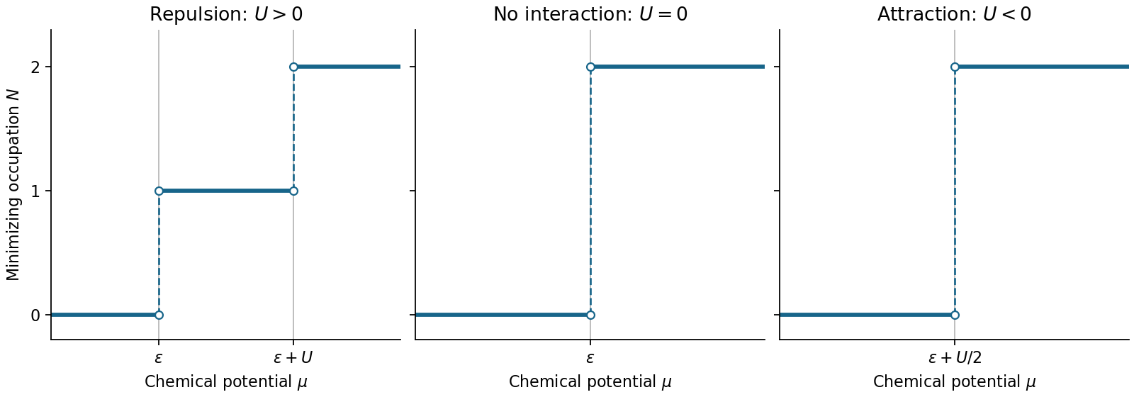
Zero-temperature occupation of a localized impurity level in a crystal with repulsive, zero and attractive interaction
. Original plots of the minimizing occupation away from degeneracy points. Dashed vertical lines mark the chemical potentials at which different occupations have equal grand energy. Their vertical segments indicate jumps, not intermediate stable states. Details. Past exam of the physics B course of the University of Cambridge 2018 Paper 2 Section A A4 Solution by Codex 0 2026-10-18
Codex 0 2026-10-18Model air as a dilute ideal gas of molecules described by the hard sphere model. The number density and mean free path areThe factor accounts for the relative motion of the colliding molecules. A molecular collision diameter has to be estimated because none is supplied. Taking , appropriate as an order-of-magnitude size for the main constituents of air, givesThus the mean free path is about , or . A slightly smaller assumed diameter gives about , illustrating the intended precision of the estimate.
Past exam of the physics B course of the University of Cambridge 2018 Paper 2 Section A A3 Solution by Codex 0 2026-10-18
Codex 0 2026-10-18Let the particle have mass , and assume its force is derived from a time-independent potential energy during the stated interval. Differentiation givesFor , choose a branch on which is real. Conservation of energy is the quickest integration of Newton's second law:The additive constant is arbitrary. For instance, the displayed expression applies directly for , and , without raising a possibly negative to a fractional power. Its derivative gives along the trajectory, as required. The second term has units of kinetic energy because has units .
For , the velocity is constant, so the potential energy is constant on the visited interval; the expression above reduces to such a constant. For , or , the particle is stationary: the trajectory only fixes to vanish at its position and does not determine the potential energy elsewhere. These exceptional cases cannot determine a unique nonconstant function.
Past exam of the physics B course of the University of Cambridge 2018 Paper 2 Section A A2 Solution by Codex 0 2026-10-18
Codex 0 2026-10-18Use absolute temperatures and . Let be the heat extracted from the ground, the heat delivered indoors, and the electrical input power. For a reversible heat pump, the entropy transferred per unit time balances:Consequently the coefficient of performance isThe requested heat delivery is a rate, since the duration is unspecified:Of this, comes from the ground and from the electricity. A coefficient of performance greater than one is consistent with conservation of energy because the heat pump transports heat as well as converting electrical energy.
Past exam of the physics B course of the University of Cambridge 2018 Paper 2 Section A A1 Solution by Codex 0 2026-10-18
Codex 0 2026-10-18For the usual hollow rectangular electromagnetic waveguide, let the propagation axis be and the interior be , . A transverse magnetic polarization has and . At a perfect conductor wall the tangential electric field vanishes. Since is tangential to all four side walls, it satisfies a homogeneous Dirichlet boundary condition around the rectangle.
Separating the transverse Helmholtz equation therefore gives the transverse magnetic mode of a rectangular waveguideA zero value of either index makes identically zero, rather than producing a nonzero field uniform along that direction. The transverse electric and magnetic fields of this TM family are obtained from transverse derivatives of , so they also vanish. Thus both TM indices must be nonzero: neither nor exists in this rectangular hollow-guide model. In contrast, transverse electric modes obey a Neumann boundary condition on and may have one zero index. The claim is about this waveguide geometry, not all possible guides.
Past exam of the physics B course of the University of Cambridge 2018 Paper 1 Section C C13 Solution by Codex 0 2026-10-18
Codex 0 2026-10-18Meaning and microscopic origin. For a Newtonian fluid, the dynamic viscosity measures tangential momentum transfer between fluid layers moving at different speeds. For the Newtonian shear considered here, , with units for . Molecular motion and collisions transport momentum across layers in a gas; intermolecular interactions contribute strongly in liquids. The resulting viscous forces oppose relative shear motion and convert organized kinetic energy to heat. The constitutive law is Newtonian and isotropic; incompressibility alone does not establish it.
Vertical force balance. Choose downward, as in the original diagram, and outward normal to the plate. In a uniform steady film, has zero advective acceleration and no along-plate pressure gradient. On a slice of thickness , the net shear force per unit face area is , while its weight per unit area is . ThereforeHere denotes the downward traction on a face with positive normal. The opposite face has the opposite traction orientation, accounting for the sign in the force difference.
Boundary conditions. At the fixed solid wall, the no-slip boundary condition is , with no normal penetration. At the free surface , neglect air shear, so and hence . The flat free surface has normal pressure , neglecting surface-curvature effects. These are a velocity condition at the wall and a stress condition at the free surface, not zero velocity at both boundaries.
The parabolic speed profile. Integrating from the shear-free surface gives . Thusand the wall condition yieldsIt is zero at the wall and largest at the free surface, where its gradient vanishes. The wall shear supports the downslope weight of the film per unit plate area.
Volume flux per unit width. Integrate through the depth:This is volume flow per unit length in , with units .
Inclining the plate. Keep normal outward from the plate and use downslope. The gravitational components are downslope and normal to the plate. For a uniform film of normal thickness , the steady slice equations areThe free-surface pressure condition givesUniform makes . The same no-slip and zero-surface-shear conditions then give the uniform gravity-driven Newtonian film,The component normal to the plate changes the hydrostatic pressure, while the tangential component drives the flow. The thickness is measured normal to the tilted plate.
The inclined-film volume flux. Integrating the new profile givesIt recovers the vertical result at and vanishes on a horizontal plate at fixed uniform depth. A varying depth, imposed pressure gradient or significant air shear would require additional terms; the solution here uses the uniform film specified by the simple draining-plate model.
Past exam of the physics B course of the University of Cambridge 2018 Paper 1 Section C C12 Solution by Codex 0 2026-10-18
Codex 0 2026-10-18Compression and stretch viewed on rotated faces. To isolate shear, take equal small principal strains , . A square with sides at to these directions becomes a rhombus: adjacent side lengths are unchanged to first order, but their right angle changes by . In axes rotated through , the same strain tensor has zero diagonal entries and off-diagonal entries of magnitude .
The pure shear from opposite principal strains therefore has engineering shear strain , not . Equal opposite principal stresses give purely tangential traction of magnitude on those rotated faces. HenceIf the compression and stretch are not equal and opposite, an additional dilatational strain remains; their deviatoric part still supplies shear.
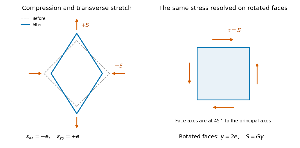
Original comparison of compression and transverse extension with the same stress resolved as shear on faces rotated through 45 degrees; deformation is exaggerated
. Details. The shaft's torsional stiffness. At radius , an end twist over length gives tangential displacement and shear angle . The local shear stress is . An annular area contributes torque , soThus torsion of a solid circular shaft givesHere is the polar second moment of area, in , not a mass moment of inertia. This is the transmitted torque magnitude; the shaft's restoring couple opposes the twist. The formula assumes small elastic shear and a circular uniform section.
Past exam of the physics B course of the University of Cambridge 2018 Paper 1 Section C C11 Solution by Codex 0 2026-10-18
Codex 0 2026-10-18The differential gravitational acceleration responsible for a tidal force is the difference between accelerations at separated points of a body. Relative to a freely falling reference point , a small offset experiencesThe tidal tensor has units ; the vector called in the source is the resulting differential acceleration, in . An actual differential force is this vector multiplied by the test mass. Measurable effects include relative motion of separated freely falling masses, radial stretching, transverse squeezing, deformation and, when self-gravity or strength is insufficient, disruption. A spatially uniform acceleration alone produces no tidal deformation.
Pinned article: Introduction to the OurBigBook Project
Welcome to the OurBigBook Project! Our goal is to create the perfect publishing platform for STEM subjects, and get university-level students to write the best free STEM tutorials ever.
Everyone is welcome to create an account and play with the site: ourbigbook.com/go/register. We belive that students themselves can write amazing tutorials, but teachers are welcome too. You can write about anything you want, it doesn't have to be STEM or even educational. Silly test content is very welcome and you won't be penalized in any way. Just keep it legal!
Intro to OurBigBook
. Source. We have two killer features:
- topics: topics group articles by different users with the same title, e.g. here is the topic for the "Fundamental Theorem of Calculus" ourbigbook.com/go/topic/fundamental-theorem-of-calculusArticles of different users are sorted by upvote within each article page. This feature is a bit like:
- a Wikipedia where each user can have their own version of each article
- a Q&A website like Stack Overflow, where multiple people can give their views on a given topic, and the best ones are sorted by upvote. Except you don't need to wait for someone to ask first, and any topic goes, no matter how narrow or broad
This feature makes it possible for readers to find better explanations of any topic created by other writers. And it allows writers to create an explanation in a place that readers might actually find it.
Figure 1. Screenshot of the "Derivative" topic page. View it live at: ourbigbook.com/go/topic/derivativeVideo 2. OurBigBook Web topics demo. Source. - local editing: you can store all your personal knowledge base content locally in a plaintext markup format that can be edited locally and published either:This way you can be sure that even if OurBigBook.com were to go down one day (which we have no plans to do as it is quite cheap to host!), your content will still be perfectly readable as a static site.
- to OurBigBook.com to get awesome multi-user features like topics and likes
- as HTML files to a static website, which you can host yourself for free on many external providers like GitHub Pages, and remain in full control

Figure 2. You can publish local OurBigBook lightweight markup files to either OurBigBook.com or as a static website.
Figure 3. Visual Studio Code extension installation.
Figure 5. . You can also edit articles on the Web editor without installing anything locally. Video 3. Edit locally and publish demo. Source. This shows editing OurBigBook Markup and publishing it using the Visual Studio Code extension. 
- Infinitely deep tables of contents:




All our software is open source and hosted at: github.com/ourbigbook/ourbigbook
Further documentation can be found at: docs.ourbigbook.com
Feel free to reach our to us for any help or suggestions: docs.ourbigbook.com/#contact