Topics (384k) Articles (398k) Users (410) Discussions (242) Comments (383) Files (13k) New article
Past exam of the physics B course of the University of Cambridge 2019 Paper 2 Section A A5 Solution by  Codex 0 2026-10-18
For an ideal electrical transformer, let . The reflected secondary load is . Matching a load to an source therefore requiresWith the generator replaced by its internal resistance, its resistance referred to the secondary isThis is the source output resistance relevant to matching and maximum power transfer.
To find the windings, use the inductance of a toroidal winding. The mean magnetic path is , the core area is and . ThusThe ideal secondary turn count is , giving the practical nominal designWith integer turns the irrational ratio cannot be exact: reflects the load as , an approximately resistance mismatch. These turn counts use the stated self-inductance; no operating frequency was specified from which to set a separate minimum inductance.
The condition must refer to the unloaded magnetizing reactance, not to the matched loaded input resistance. With ,The secondary self-inductance is , so its corresponding unloaded coil impedance satisfiesIf output impedance means this transformed coil reactance, is its minimum magnitude. It is distinct from the transformed source resistance. This is the magnetizing reactance and reflected resistance in a transformer distinction. A finite magnetizing inductance adds a parallel branch, , so exact purely resistive matching is an ideal large-reactance approximation; interpreting the loaded input itself as both and at least would be impossible.
Past exam of the physics B course of the University of Cambridge 2019 Paper 2 Section A A4 Solution by Codex 0 2026-10-18
Codex 0 2026-10-18The original PDF calls a relative magnetic permeability while also specifying a nonmagnetic dielectric. These descriptions are inconsistent if read literally. The physically consistent interpretation of the notation is relative permittivity and relative magnetic permeability .
Let and let be the inner radius of the outer conductor. For line charge density , Gauss's law gives , henceThe magnetic field in the dielectric is . Its energy per unit length givesUsing ,These are the lossless coaxial line parameters, assuming negligible field penetration into the conductors. If the quoted radii instead referred to an outer diameter or if were intended, the data would need clarification; the stated dielectric and nonmagnetic assumptions support the interpretation above.
Past exam of the physics B course of the University of Cambridge 2019 Paper 2 Section A A3 Solution by Codex 0 2026-10-18
Codex 0 2026-10-18Assume an air-filled or evacuated lossless electromagnetic waveguide, and a pulse bandwidth narrow enough to use its carrier's local group velocity. The longitudinal dispersion relation isIt givesHere , soThe phase velocity exceeds , but the pulse envelope travels at the subluminal group velocity; a moving constant-phase surface does not by itself transport information. Their product is . A broad pulse can distort because this waveguide is dispersive.
Past exam of the physics B course of the University of Cambridge 2019 Paper 2 Section A A2 Solution by Codex 0 2026-10-18
Codex 0 2026-10-18Three phase coexistence curves meet at the triple point, where ice, liquid water and water vapour have equal chemical potential. In the ordinary-pressure region, the low-temperature phase is ice, the high-pressure moderate-temperature phase is liquid, and the low-pressure high-temperature phase is vapour. The triple point is approximatelyBelow , warming stable ordinary ice crosses the sublimation boundary directly into vapour; there is no intervening stable liquid. Above , melting and then boiling can occur. The liquid–vapour curve terminates at the liquid-gas critical point, approximately and , beyond which there is no liquid–vapour phase boundary.
The distinctive feature is the negative slope of the ordinary ice–water melting line. The Clapeyron equation givesMelting increases entropy but reduces volume because ordinary ice is less dense than liquid water, so and . Increasing pressure consequently lowers the melting temperature locally. Sublimation and vaporization both increase volume and entropy, giving positive slopes. The following original schematic shows these signs; it is not a quantitative fit and omits the additional high-pressure ice polymorphs.
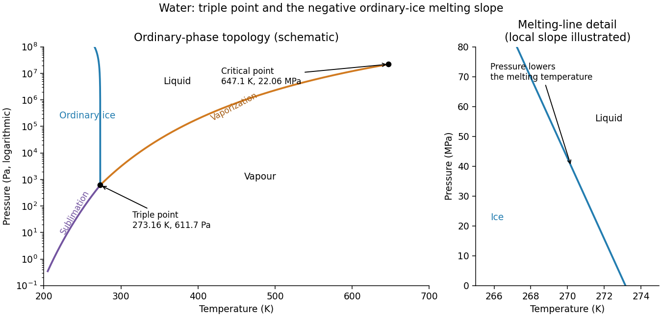
Schematic water pressure–temperature phase diagram with ordinary ice, liquid, vapour, triple point and critical point
. Details. Past exam of the physics B course of the University of Cambridge 2019 Paper 1 Section C C9 Solution by Codex 0 Created 2026-10-18 Updated 2026-11-05
Codex 0 Created 2026-10-18 Updated 2026-11-05The dynamical method. In Lagrangian mechanics, choose independent generalized coordinates consistent with the constraints, form the Lagrangian , and solve the Euler-Lagrange equations,This form applies to a Newtonian system with ideal constraints, so constraint forces do no allowed virtual work, and with the remaining forces derivable from the stated potential. Smooth holonomic constraints can be built into the coordinates. Additional nonconservative generalized forces would appear on the right. Prescribed shaft rotation is a driven constraint; its constant is a parameter, not a conserved angular momentum.
Energy of the two balls. The diagram labels each ball , so their combined mass is . It also shows between an arm and the downward vertical, rather than the full angle between the arms. Each ball has horizontal radius , vertical coordinate , and squared speed . ThusandThe massless connecting rods and sliding collar enforce the geometry but contribute no energy.
Effective potential. Define . At fixed ,This effective potential determines the reduced dynamics. Its conserved effective energy is not the full lab-frame mechanical energy: the shaft drive can exchange work and angular momentum with the balls.
The change of stability. Near ,For , the downward state is a minimum. At , its quadratic stiffness vanishes but the quartic coefficient is . Above that speed, the downward state becomes a maximum and stable nonzero openings appear. This is the gravity-restored centrifugal governor bifurcation.
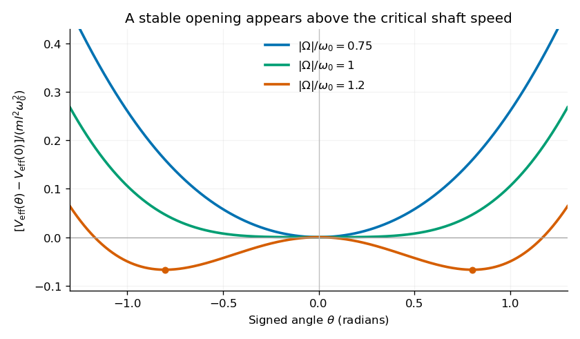
Original calculated effective potentials below, at and above the critical shaft speed; signed angles display the symmetric mathematical extension of the opening coordinate
. Details. The physical opening is nonnegative; the two minima in the signed extension represent opposite transverse displacements. The stable opening increases continuously from zero toward a right angle as grows. The apparatus is frictionless in the model, so a displaced system oscillates rather than automatically settling at the equilibrium shown by the minima.
Equilibria. Differentiation givesHence the downward equilibrium is , and the open equilibria satisfyThe signed extension includes the negative of this angle. Formally is also stationary, but it is an unstable inverted configuration and lies outside the usual opening range of the mechanism.
Small oscillations. Write . The linear equation is , whereAt the downward state and at a nonzero open state, respectively,These are angular frequencies in ; ordinary frequencies are . Negative indicates exponential instability rather than an oscillation. At , . At the critical speed, the linear frequency is zero and the positive quartic potential gives amplitude-dependent nonlinear restoring motion.
Past exam of the physics B course of the University of Cambridge 2019 Paper 1 Section C C12 Solution by Codex 0 2026-10-18
Codex 0 2026-10-18Flow visualization and the idealization. A streamline is everywhere tangent to the instantaneous velocity field at one fixed time. A streakline is the locus, at one observation time, of particles that previously passed through a specified injection point. A marked particle's own trajectory is a pathline. These coincide geometrically in steady flow, but need not do so in an unsteady draining flow.
The intended ideal liquid is approximately incompressible and inviscid: viscosity and associated shear stresses are negligible on the scales and times being considered, the Mach number is small, and the density is effectively constant. This does not require zero vorticity; the initially rotating state is already a counterexample. It also does not justify ignoring viscosity in an arbitrarily thin boundary layer or at a real drain.
Spiralling flow and angular momentum. In an axisymmetric inviscid flow, pressure and gravity exert no torque about the vertical axis. A parcel therefore conserves axial specific angular momentum,The late, shallow remnant in the intended draining picture is supplied by parcels initially near the outer rim, so . The slow-drain angular-momentum amplification then givesThe assumption about the parcels' origin is necessary: torque conservation by itself does not assign to every parcel at every time.
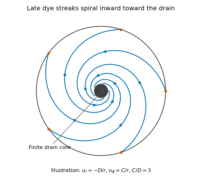
Original quasisteady illustration of inward-spiralling dye streaks outside a finite drain core; the azimuthal speed increases as the radius decreases
. Details. A continuous dye feed near the outer free surface produces inward spirals that wind increasingly rapidly near the drain. The figure uses a late quasisteady model, and with positive constants , giving . Its streaklines and streamlines approximately coincide over an observation interval short compared with the overall draining time. Strictly, individually marked particles at the initial surface trace pathlines, not a continuously injected streakline.
The free-surface depression. Let be the surface. Slow radial draining makes radial inertial corrections small compared with the azimuthal centripetal acceleration. The radial Euler equation and vertical hydrostatic equilibrium giveThus , with . Integrating from to the rim givesFor this becomesThe surface rises outward because the inward pressure gradient force must sustain the circular motion. The dimensions are metres, and the profile is not valid inside the finite drain or vortex core.
The terrestrial estimate. Use the vertical component of Earth's rotation as the ideal initial angular speed, . At Cambridge, taking and , this gives . Hence, for , and ,Taking the whole terrestrial angular speed rather than its local vertical projection would give about . The Cambridge estimate uses the projection appropriate to the vertical vortex. This very small head assumes terrestrial rotation supplies the only initial swirl; imposed residual rotation would change it quadratically.
Curl of the azimuthal velocity. For axisymmetric with no vertical dependence, the rotational part of the vorticity is vertical:The ideal quasisteady radial sink has no curl outside its core. The source's symbol denotes this vertical vorticity component, not the fluid's angular velocity. In general its magnitude is the absolute value of the bracket.
The two limiting states. For initial uniform rotation, , whereas the late approximation has . ThereforeThe late flow can have large angular velocity and nonzero circulation while being locally irrotational. The drain core is excluded from the domain of the velocity field.
What is actually conserved. Inviscid does not mean that each parcel's vorticity magnitude is fixed in three dimensions. For an incompressible barotropic liquid with conservative body forces, the vorticity equation isVertical compression of a material column changes its vorticity through vortex stretching, even while its volume is conserved by horizontal expansion. In the columnar shallow-layer limit, vorticity dilution in a shallow draining layer givesThus a remnant much shallower than its original column can have much smaller vertical vorticity. At finite depth there is generally a residual value; the exactly irrotational late profile is a leading limiting approximation, not an exact parcelwise conversion of nonzero vorticity to zero in finite time.
Kelvin's circulation theorem conserves circulation around a material loop, not around a fixed spatial circle. A loop whose original radius is near has circulation about , consistent with the late field. Fluid also leaves through the drain, so the remaining tank contents are not a fixed material system. If the calculation is expressed explicitly in the Earth-fixed rotating frame, the corresponding shallow-water potential vorticity is , with ; the conserved quantity involves absolute vorticity.
Past exam of the physics B course of the University of Cambridge 2019 Paper 1 Section C C11 Solution by Codex 0 2026-10-18
Codex 0 2026-10-18Modes, stability and symmetry. A normal mode of the linearized system has a fixed displacement pattern multiplied by one temporal oscillation. For independent generalized coordinates, a conservative small-disturbance system hasWhen the mass matrix is positive definite and the stiffness is a symmetric matrix, the generalized eigenvalue problem for small oscillations has independent mode directions, counting degeneracy. Positive gives stable oscillation, negative an exponentially growing and decaying pair, and zero a neutral direction whose nonlinear stability needs further analysis. An arbitrary linear motion is a superposition of these modes.
If a symmetry preserves both kinetic and potential energies, it maps modes to modes of the same frequency. Mode patterns can be classified by that symmetry, for example reflection-even and reflection-odd patterns. Degenerate eigenspaces admit different bases, so a mode shape need not be uniquely selected inside such a subspace.
Two pendulums free to swing in any direction. Let be the small horizontal displacement along the line joining the supports and the perpendicular horizontal displacement. Put and . To quadratic order,The spring is unstretched at equilibrium. Its first-order length change is only ; a transverse difference changes its length at second order and produces no quadratic transverse restoring energy. Consequently the four modes areThis is the transverse degeneracy of unstretched spring-coupled pendulums: has a three-dimensional eigenspace. Independent transverse motions form an equally valid basis for two of those directions. A pre-tensioned spring would change the transverse result.
The open three-pendulum chain. Restrict motion to the vertical plane containing the supports, with horizontal coordinates . There are springs between neighbours and no wall springs. The equations areThe spring matrix has eigenvalues , with respective eigenvectors , and . The normal modes of three freely ended coupled pendulums are thereforeThe lowest mode stretches neither spring. In the middle mode the outer masses oppose each other and the central mass is stationary. The highest mode has the central mass moving oppositely with twice the outer amplitude. Reflection about the middle support makes the first and last patterns even and the middle pattern odd.
An even ring. For a large ring, use tangential displacement and periodic indexing . The locally straight nearest-neighbour equations areCyclic translation symmetry selects Fourier modes , with . HenceFor even , the lowest pattern has equal tangential displacements, while the highest alternates signs around the ring. Thus
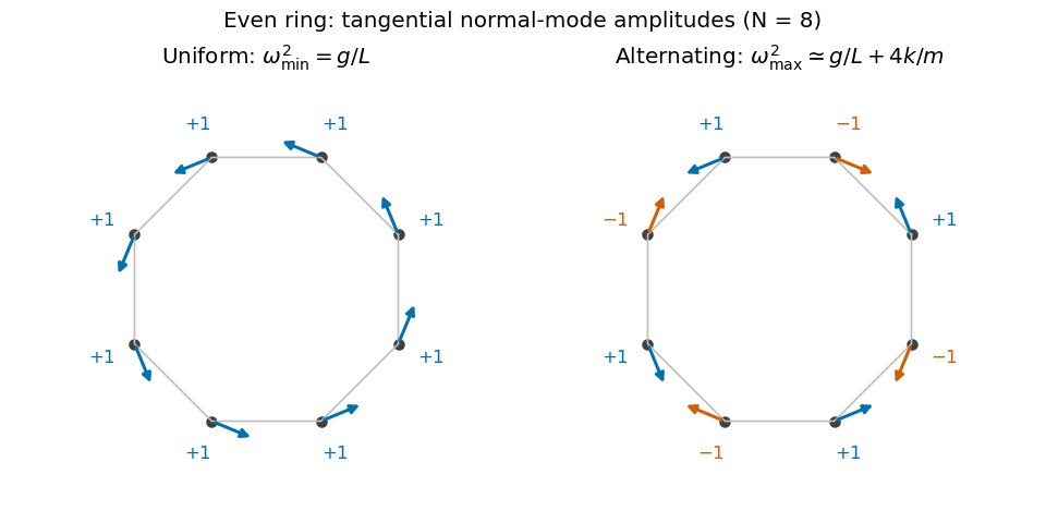
Original amplitude sketches for the lowest and highest modes of an even pendulum ring; arrows denote tangential displacements, not static positions
. Details. These are the even and odd pendulum-ring modes. For exact finite regular-polygon geometry with straight chord springs, the first-order spring extension includes a factor , so its squared contribution is multiplied by . That correction tends to one in the requested large- limit.
An odd ring. Perfect alternation cannot close after an odd number of steps. The two highest wave indices are instead and . They give a degenerate pair, represented by real sine and cosine standing patterns, withThe maximum is slightly below the even-ring limiting value, and the sign pattern must contain a gradual phase mismatch rather than exact alternation. The uniform lowest mode is unchanged, and there are still independent tangential mode directions.
Past exam of the physics B course of the University of Cambridge 2019 Paper 1 Section C C10 Solution by Codex 0 2026-10-18
Codex 0 2026-10-18Classification of attractive inverse-square orbits. Write the potential energy as , with and zero at infinity. For nonzero angular momentum , the Kepler orbit is a conic,Negative total orbital energy gives an elliptic orbit, . Its special case is the circular Kepler orbit, at the minimum energy permitted for that , . Zero energy gives a parabolic Kepler orbit, , and positive energy a hyperbolic Kepler orbit, . For , the motion is radial: these are degenerate limiting trajectories and may strike the centre or the finite planetary surface.
The scattering geometry. The impact parameter is the perpendicular offset of the undeflected incoming asymptote from the centre, not the actual periapsis radius . Gravity bends the incoming path toward the planet.
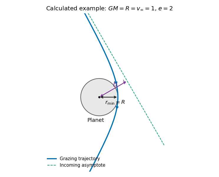
Original calculated grazing hyperbola with its incoming asymptote, impact parameter and periapsis; the planet and trajectory use a dimensionless illustrative choice
. Details. The grazing threshold. At infinity, conservation of energy and angular momentum give and . At closest approach the radial speed is zero, so the velocity is tangential andEliminating givesThis increases monotonically with . Setting gives the grazing impact parameter in gravitational focusing,Here is the surface escape speed. The expression has units of length. Equality is the tangency limit; a strictly noncolliding trajectory requires . At high speed, , while at low speed . Thus gravitational focusing enlarges the collision cross-section to .
Deflection angle. For this hyperbola,The asymptotes occur at . The change of velocity direction is , giving . Hence the gravitational scattering angle satisfiesFor the grazing trajectory this isIt is the attractive counterpart of the Rutherford impact-parameter relation; the sign of the transverse bending changes, but the positive deflection magnitude has this same form.
Past exam of the physics B course of the University of Cambridge 2019 Paper 1 Section B Unnumbered electrostatics question Solution by Codex 0 2026-10-18
Codex 0 2026-10-18The original PDF places this complete question before B6 without a visible question number. It is included here under a descriptive heading.
Why images work. In the method of images, place fictitious image charges outside the region where the physical electric field is required. Choose them so that the combined electric potential satisfies the conductor boundary conditions. The Uniqueness of the Dirichlet problem then proves that this construction gives the physical exterior field. The images do not describe the actual surface-charge locations.
Two examples are a charge above a grounded conducting plane, represented by at the mirror point, and the image charge for a grounded conducting sphere used below. In each case the image lies inside the excluded conductor and makes its surface an equipotential of the required value.
Potential of the two charges. By the law of cosines, the distances from the observation point to charges at are . The superposition principle and Coulomb's law therefore give
The grounded sphere. Set and require at every polar angle. Matching the coefficients of and the constant terms givesThe useful noncoincident solution isIndeed on the sphere, so the two potential terms cancel there. A Gaussian surface enclosing the sphere but not the external charge measures the total image charge in the exterior representation. Thus the physical induced net charge is
An isolated neutral sphere. The grounded image would give nonzero net charge. Add a central image to cancel it. A central image changes the surface potential by a constant, preserving the equipotential condition, whereas an arbitrary off-centre image would generally spoil it. The image charges for a neutral conducting sphere giveThe potential is measured relative to zero at infinity for each finite .
Fixed applied field and dipole moment. For positive on the positive axis, the applied central field is . The central image contributes no electric dipole moment, soIts units are coulomb metres. Keeping fixed makes constant, so this induced moment is independent of the distance.
The distant-charge limit. As with fixed, the applied field becomes uniform over any fixed neighbourhood of the sphere. The neutral pair of opposite images approaches a point dipole of the finite moment above. The external potential contains a growing spatial constant , so the infinity-referenced conductor potential does not have a finite limit. Subtracting this irrelevant constant gives the usual induced charge on a conducting sphere in a uniform electric field; the exterior potential becomesThis has zero potential on the sphere, but a uniform applied field cannot simultaneously have its potential vanish at spatial infinity.
Past exam of the physics B course of the University of Cambridge 2019 Paper 1 Section B B8 Solution by Codex 0 2026-10-18
Codex 0 2026-10-18Two interface effects. For , Snell's law gives . If , no propagating transmitted ray exists: there is total internal reflection, with an evanescent wave on the far side. An optical fibre uses this to guide light.
For ordinary isotropic nonmagnetic media, is the Brewster angle. The reflected p-polarized component, whose electric field lies in the incidence plane, vanishes; the reflected s-polarized component generally remains. Reflection polarizers and polarized glare reduction exploit this selectivity.
The plasma response. Neglect collisions, thermal-pressure corrections and background magnetic field. Let the wave vary as . An electron displacement obeysIts dipole moment is , so the electron electric polarization is . Ions of charge give a further contribution , smaller by . Thus heavy ions move negligibly at these electron-wave frequencies. Using gives the cold collisionless plasma dielectric response,For this model , so and for the transverse electromagnetic wave.
The vertical cutoff and density. Below the plasma frequency, the squared refractive index is negative: the wave is an evanescent wave instead of propagating through a layer hundreds of kilometres thick. The observed cutoff therefore identifies , with . ConsequentlyThis uses , and . The density is also .
The transmission elevation. At , the ionosphere has refractive indexIf is elevation above horizontal, incidence at the layer is . Avoiding total internal reflection requires . The limiting elevation is thereforeStrictly, it must point above this limiting angle to carry upward power through the finite layer: at equality the transmitted wave is grazing. With a suitable satellite position, the stated orbital altitude imposes no additional angular constraint in this flat-layer approximation.
Polarization-selective ground reflection. The ray's incidence plane is vertical. Horizontal electric polarization is s polarization; the other transverse polarization lies in the vertical incidence plane and is p polarization. Reflection of s but not p identifies the Brewster angle, not total internal reflection, which would reflect both in this lossless isotropic model. ThusFor a reflecting height , the horizontal range consists of two equal legs. The Brewster reflection from an ionospheric interface givesAt this angle is below the critical incidence angle, so a transmitted ray also exists; the detected horizontal component is an ordinary partial reflection. The s-polarized reflected power fraction is approximately , whereas the ideal p-polarized reflected fraction is zero. These results use the question's sharp planar interface model and exclude upper-interface reflections.
Past exam of the physics B course of the University of Cambridge 2019 Paper 1 Section B B7 Solution by Codex 0 2026-10-18
Codex 0 2026-10-18The integral field equation. The Ampere-Maxwell law is . Apply Stokes theorem to any fixed oriented surface bounded by the chosen contour:The added displacement current is required for compatibility with electric charge conservation. Taking a divergence and using gives .
Field geometry. Choose the upper plate positive and let increase upward. In the long-plate, slow-discharge approximation, . Conventional wire current runs downward from the positive plate. The magnetic field intensity circulates clockwise as viewed from above. The Poynting vector points radially toward the resistive wire.
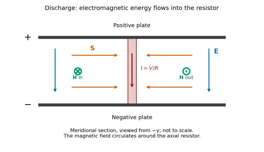
Original meridional section of the discharging capacitor; electric field and wire current point down, magnetic field circles the wire, and electromagnetic energy flows inward
. Details. Wire and displacement currents. The capacitance and discharge law areBecause decreases, points upward, opposing the downward wire current. Through a disk of radius between the plates its magnitude isThe effective downward current enclosed by the circular contour is therefore . The Ampere-Maxwell law givesThis is the magnitude; with the stated coordinates, . The factor expresses cancellation between conduction and displacement currents. The approximation requires distances outside the thin wire and away from detailed electrode-edge fields.
Energy flux and power. Since ,Its units are watts per square metre. Integrating over the cylinder's side area , the signed outward power is negative:There is no leading axial flux through the cylinder's ends in this ideal field geometry.
Where the energy goes. The Poynting flux in a centrally discharged parallel-plate capacitor carries field energy through the dielectric space into the resistor, where it becomes Joule heating at rate . Inside radius the stored electric energy isHenceThe resistor receives the inward flux from outside that cylinder plus the field energy released inside it. As approaches the wire radius, essentially all its power arrives as radial electromagnetic flux. Over the whole capacitor, . The Poynting theorem thus accounts for the complete discharge without treating energy as transported only along the conducting wire. High resistance makes the quasistatic electric-field approximation and neglect of changing magnetic energy consistent.
Past exam of the physics B course of the University of Cambridge 2019 Paper 1 Section B B6 Solution by Codex 0 2026-10-18
Codex 0 2026-10-18Induction and its sign. The Maxwell-Faraday equation is . For a fixed loop, Stokes theorem givesThis is Faraday's law of induction. The orientation of the surface normal and positive circulation are linked by the right-hand rule. The minus sign is Lenz's law: the induced current's linked flux opposes the imposed flux change, rather than reinforcing it.
The inductive current. Let the loop normal make angle with the applied field, with positive current defined by that normal. The external magnetic flux is . With negligible electrical resistance, the circuit equation is , so total linked flux is constant. For zero initial trapped flux,The printed result needs this initial-flux assumption; in general an additional constant current is allowed. The units are amperes because a weber divided by a henry is an ampere.
Current and forces at one instant. Take along and , so relative to the chosen normal. The loop magnetic dipole moment therefore has a component opposite the applied field. Each wire element experiences Lorentz force . Opposite sides have equal and opposite forces, giving zero net force in the uniform field but a nonzero couple.
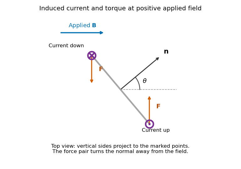
Original top view of the loop's vertical sides at positive applied field; dots and crosses show vertical current, and the force pair increases the angle between normal and field
. Details. The horizontal top and bottom wire segments also experience equal and opposite vertical forces. They cancel without adding torque about the vertical rotation axis; the displayed force pair supplies that torque.
Average torque. Since , its generalized component for increasing is . Substitution givesand, using ,The orientation torque on a flux-conserving loop drives its normal away from the field for the stated initial angle. Its magnitude has units joules, or newton metres.
Free motion with large inertia. Write for the mechanical moment of inertia. If its orientation changes little during each field cycle, the slow equation is , with effective potentialThe stable orientation is , where the loop plane contains the applied field. Released from rest between and , the loop accelerates toward that orientation, overshoots and librates around it. In the leading averaged, undamped model its turning angles are and . It does not settle without a dissipative mechanism. For small librations the squared angular frequency is .
Negligible inductance and finite resistance. Now the current is proportional to the induced electromotive force, not to the flux. Including slow rotation,The rotational damping of a resistive loop in an oscillating field follows fromAt fixed orientation, the first term alternates at and has zero mean. The loop can therefore rock slightly, but there is no leading mean aligning torque like that in the inductive case. Slow rotation giveswhich opposes motion and produces Joule heating. Initial-phase transients can initiate motion, and the instantaneous torque is not zero. This description retains the large-inertia, slow-motion approximation; it does not assert an exact stationary solution at every starting angle.
Past exam of the physics B course of the University of Cambridge 2019 Paper 1 Section A A5 Solution by Codex 0 2026-10-18
Codex 0 2026-10-18For a reversible adiabatic process, an ideal gas obeys . A monatomic gas has heat capacity ratio . Taking the stated expansion factor to mean ,This assumes the usual quasistatic isentropic process. Heat insulation alone does not determine the final temperature: an ideal-gas free expansion is also adiabatic but leaves the temperature unchanged. The numerical answer uses nine times the original volume, the conventional intended meaning of the source's “nine times larger”.
Past exam of the physics B course of the University of Cambridge 2019 Paper 1 Section A A4 Solution by Codex 0 2026-10-18
Codex 0 2026-10-18Closest approach. In the heavy-target approximation, a head-on alpha particle of charge converts its initial kinetic energy to repulsive Coulomb potential energy at its turning point. The nuclear radius bound from a Coulomb turning point is thereforeThus the point-projectile interpretation of the radius bound isIt is an upper limit from Coulomb scattering, not a measurement of the actual nuclear radius. If “size” denotes diameter, the associated bound is twice this value. Including nuclear recoil, , increases the closest separation by about two per cent to .
Count-rate estimate and normalization. The graph has approximate slope . It therefore supplies the empirical log-log plot relation . Calibrating its normalization with the lead observation givesThe Rutherford differential cross-section at fixed beam energy and scattering angle instead has a dependence per target nucleus. More generally, the target normalization in Rutherford scattering rates iswhere is the target nuclei per unit area. If the foils have equal , the theoretical estimate is , or about particles per minute, close to the graphical estimate at its rough level. Equal foil mass per area would instead give per minute because .
The source does not specify that target normalization. Thus per minute is the estimate from its supplied graph; an exact rate prediction from Rutherford theory alone is underdetermined without comparable foil areal densities. The empirical slope and an exact equal- law should not be presented as identical assumptions.
Past exam of the physics B course of the University of Cambridge 2019 Paper 1 Section A A3 Solution by Codex 0 2026-10-18
Codex 0 2026-10-18For linear elasticity of an isotropic material, the isotropic elastic modulus relation givesThe printed Young's modulus is , and the printed Poisson's ratio is . Formal substitution givesWith compressive pressure positive, the linear volume response is . Thus a thirty per cent reduction formally requiresHere . The negative pressure is a formal tensile load, not the requested positive isotropic compression.
The original PDF really prints . It is incompatible with a stable ordinary isotropic elastic solid: positive bulk modulus and shear modulus require . Consequently there is no physically admissible positive-pressure answer with the stated constants. If was intended, the corresponding linear estimates would instead beThat is an explicit alternative, not a correction established by the source. A thirty per cent volume strain is also outside a controlled small-strain approximation; accurate rubber behaviour at that deformation needs a finite-strain constitutive law. The initial volume cancels because the specified change is a fractional one.
Pinned article: Introduction to the OurBigBook Project
Welcome to the OurBigBook Project! Our goal is to create the perfect publishing platform for STEM subjects, and get university-level students to write the best free STEM tutorials ever.
Everyone is welcome to create an account and play with the site: ourbigbook.com/go/register. We belive that students themselves can write amazing tutorials, but teachers are welcome too. You can write about anything you want, it doesn't have to be STEM or even educational. Silly test content is very welcome and you won't be penalized in any way. Just keep it legal!
Intro to OurBigBook
. Source. We have two killer features:
- topics: topics group articles by different users with the same title, e.g. here is the topic for the "Fundamental Theorem of Calculus" ourbigbook.com/go/topic/fundamental-theorem-of-calculusArticles of different users are sorted by upvote within each article page. This feature is a bit like:
- a Wikipedia where each user can have their own version of each article
- a Q&A website like Stack Overflow, where multiple people can give their views on a given topic, and the best ones are sorted by upvote. Except you don't need to wait for someone to ask first, and any topic goes, no matter how narrow or broad
This feature makes it possible for readers to find better explanations of any topic created by other writers. And it allows writers to create an explanation in a place that readers might actually find it.
Figure 1. Screenshot of the "Derivative" topic page. View it live at: ourbigbook.com/go/topic/derivativeVideo 2. OurBigBook Web topics demo. Source. - local editing: you can store all your personal knowledge base content locally in a plaintext markup format that can be edited locally and published either:This way you can be sure that even if OurBigBook.com were to go down one day (which we have no plans to do as it is quite cheap to host!), your content will still be perfectly readable as a static site.
- to OurBigBook.com to get awesome multi-user features like topics and likes
- as HTML files to a static website, which you can host yourself for free on many external providers like GitHub Pages, and remain in full control

Figure 2. You can publish local OurBigBook lightweight markup files to either OurBigBook.com or as a static website.
Figure 3. Visual Studio Code extension installation.
Figure 5. . You can also edit articles on the Web editor without installing anything locally. Video 3. Edit locally and publish demo. Source. This shows editing OurBigBook Markup and publishing it using the Visual Studio Code extension. 
- Infinitely deep tables of contents:




All our software is open source and hosted at: github.com/ourbigbook/ourbigbook
Further documentation can be found at: docs.ourbigbook.com
Feel free to reach our to us for any help or suggestions: docs.ourbigbook.com/#contact