Topics (384k) Articles (398k) Users (410) Discussions (242) Comments (383) Files (13k) New article
Past exam of the physics B course of the University of Cambridge 2021 Paper 1 Section A A5 Solution by  Codex 0 2026-10-18
For the intended reversible adiabatic process, an ideal gas obeys . A monatomic gas has heat capacity ratio , soThe required extra assumption is that “adiabatic” denotes the usual quasistatic isentropic process. Absence of heat transfer alone would not fix the final temperature: an ideal gas undergoing free expansion into vacuum is also adiabatic but leaves its temperature unchanged.
Past exam of the physics B course of the University of Cambridge 2021 Paper 1 Section A A4 Solution by Codex 0 2026-10-18
Codex 0 2026-10-18Under a uniform compressive pressure , each normal stress is . The isotropic Hooke's law gives each longitudinal strain asThus . By the definition of bulk modulus, , so the isotropic elastic modulus relation isPositive finite Young's modulus and bulk modulus requireThe incompressible limit is with at finite . If positivity of the shear modulus is also imposed, the full stable isotropic range is . Negative Poisson's ratio is not ruled out; the displayed bulk-modulus relation alone supplies the upper bound.
Past exam of the physics B course of the University of Cambridge 2021 Paper 1 Section A A3 Solution by Codex 0 2026-10-18
Codex 0 2026-10-18Use local east, north and upward unit vectors at the equator, with Earth's rotation . The parcel starts at rest relative to the ground. To first order in , its unperturbed vertical velocity is and its fall time from height isThe Coriolis acceleration is . Since north crossed with downward points west, its negative points east:Integrating with gives the equatorial Coriolis deflection in free fall,For , and , andThis neglects air resistance, variation of over the fall, and terms of order . The measured local already includes the background centrifugal correction. “Stationary” is interpreted as hovering above a fixed ground location, not being stationary in an inertial frame.
Past exam of the physics B course of the University of Cambridge 2021 Paper 1 Section A A2 Solution by Codex 0 2026-10-18
Codex 0 2026-10-18The principal moments of inertia are the eigenvalues of the symmetric inertia tensor. In units of , its characteristic determinant isTherefore the requested algebraic answer isAn orthonormal basis of principal axes is , , and ; the last two span the degenerate eigenspace and may be replaced by any orthonormal basis of it.
There is a physical inconsistency in calling the supplied matrix a rigid body's inertia tensor. The moment-of-inertia triangle inequalities require each principal moment to be no greater than the sum of the other two. Here . In principal coordinates, cannot be negative for a nonnegative mass distribution. Thus the eigenvalue calculation is well defined, but no ordinary rigid mass distribution realizes this tensor. The positive second-moment matrix test for an inertia tensor makes the same obstruction explicit.
Past exam of the physics B course of the University of Cambridge 2021 Paper 1 Section A A1 Solution by Codex 0 2026-10-18
Codex 0 2026-10-18For the intended ideal Venturi effect, take steady flow, incompressible flow, negligible viscous losses, and the same height at the two stations shown. The Bernoulli equation along a streamline givesUsing water mass density ,Thus the outlet pressure is lower by . The increased kinetic energy per unit volume comes from the drop in pressure.
The source's assumption of laminar flow alone does not imply negligible viscosity or losses. The numerical result uses the usual lossless Bernoulli equation approximation, with the quoted speeds interpreted as representative streamline speeds. A real tube with significant viscous losses requires additional data; in a uniform-velocity energy balance its pressure drop would include an extra positive loss term.
Past exam of the physics B course of the University of Cambridge 2019 Paper 2 Section C C13 Solution by Codex 0 2026-10-18
Codex 0 2026-10-18Temperature as an equilibrium relation. Classical thermodynamics begins with the zeroth law of thermodynamics: thermal equilibrium is transitive. A thermometer can therefore assign a common empirical temperature to systems in mutual thermal equilibrium. Different thermometer properties initially give different monotone empirical scales; a resistance reading by itself does not define the absolute scale.
The Second law of thermodynamics provides a substance-independent thermodynamic scale. A reversible engine operating between reservoirs has a heat ratio depending only on their temperatures. One chooses absolute temperature so that , with the positive heat magnitudes. Its reversible efficiency is . Equivalently, reversible heat defines entropy through . For an equilibrium simple compressible system,Classical thermodynamics uses this relation without needing a microscopic account of entropy. A dilute-gas thermometer realizes an empirical scale approaching the thermodynamic scale after corrections for nonideal behavior.
Statistical meaning of the same derivative. In the microcanonical description, an equilibrium energy shell containing accessible states has . Its statistical temperature is consequentlyTo see why this is an equilibrium temperature, let two weakly coupled systems exchange a small energy while their total energy stays fixed. The combined multiplicity is . Maximizing its logarithm giveswhich is equality of the two inverse temperatures. Stability requires the total entropy maximum, not only stationarity. The overwhelmingly dominant macrostate in a large system therefore realizes the thermodynamic equilibrium condition.
A large reservoir gives a small subsystem the canonical probabilities , with . In that ensemble, and agree with macroscopic thermodynamic relations in their usual equilibrium regime. The equipartition identity for a classical dilute monatomic gas, , is a useful operational connection between microscopic motion and temperature, but is not a universal definition: quantum modes need not obey equipartition, and a system away from equilibrium need not have one temperature at all.
For finite systems one must specify the entropy convention and energy resolution; surface and fluctuation corrections can distinguish definitions that agree in the ordinary thermodynamic limit. Bounded-energy population-inverted systems can also have a negative entropy derivative and hence a negative statistical temperature. That possibility lies outside an ordinary positive-temperature ideal-gas thermometer; it does not mean temperature is merely an arbitrary average kinetic energy.
Obtaining the energy–temperature conversion. The Boltzmann constant connects entropy measured in with the dimensionless logarithm of a state count. Historically it could be determined from the ideal gas law : measure the molar gas constant and independently determine the Avogadro constant , then obtain . The independent particle-number determination matters; using alone would not fix energy per particle.
An electrical method uses Johnson-Nyquist noise. A resistor of resistance at known temperature has, in the classical range , a one-sided open-circuit voltage-noise spectrum . Over a calibrated flat bandwidth ,A practical measurement uses an equilibrium resistor, a calibrated low-noise amplifier and a known transfer function, subtracts or independently characterizes amplifier noise, and replaces a nominal bandwidth by the actual effective noise bandwidth. Varying temperature and fitting the mean-square voltage is more informative than treating one amplified voltage sample as the thermal variance. Other primary methods relate temperature to sound speed in a dilute gas or to calibrated particle diffusion and mobility.
There is a historically relevant unit-definition qualification: by the date of this exam, the revised SI had already taken effect on 20 May 2019. The kelvin is now defined by fixingThe same experiments now realize or compare thermodynamic temperatures using this fixed constant, whereas historically they measured the conversion constant on an independently defined temperature scale. The physical distinction between equilibrium temperature and microscopic state counting is unchanged.[ref]
https://www.bipm.org/en/measurement-units/. BIPM, SI definitions effective from 20 May 2019 and fixed Boltzmann constant
Past exam of the physics B course of the University of Cambridge 2019 Paper 2 Section C C12 Solution by Codex 0 2026-10-18
Codex 0 2026-10-18Configuration count. Choose the end-to-end direction as positive and let count rightward and leftward links. ThenA configuration is determined by choosing the positions of its leftward links, soThe counts must be nonnegative integers; in particular, allowed signed extensions occur in steps of . If distance means with neither direction selected, there are two corresponding sets for , adding a factor of two. That constant does not affect the tension. There is no excluded-volume penalty in this one-dimensional idealized count.
Entropy from the multiplicity. Put , so . Applying the leading Stirling's approximation to all three large factorials givesTerms subleading in , including logarithmic factorial prefactors, have been omitted consistently. Expanding near zero extension givesStretching reduces the number of available configurations and hence the entropy.
Tension and the range of Hooke's law. The model assigns no extension-dependent internal energy. At fixed temperature, the externally applied tension is . Differentiating the full leading entropy givesIt is the external force needed to oppose the chain's restoring entropic force. Only when can one put , yieldingThe paper's displayed linear law therefore requires this small-extension approximation, which is not explicitly stated in its premise . It is not the exact force law up to full extension. The entropic spring constant grows with temperature because stronger thermal disorder makes a given reduction in configurational entropy cost more free energy. This is the one-dimensional entropic chain force-extension relation.
A sparse number of backward links. Write , so and . Exactly,For fixed and large , each numerator factor approaches , givingMore precisely, the logarithm of the product is . A small relative error in the multiplicity requires ; merely need not make the omitted product close to one. The weaker sparse-link condition does suffice for the leading entropy density and leading high-extension tension. These are sparse backward links near full chain extension.
Tension in that limit. In the overlap regime , use Stirling also for :ThusThe full leading entropy would give , which has the same dominant logarithm when .
Approaching full extension. The continuum force law diverges logarithmically as , or . One must not literally apply Stirling to a zero factorial: at the discrete endpoint there is exactly one directed configuration, , and its entropy is zero. A continuous fixed-extension derivative is not defined at that endpoint.
An independent force-ensemble calculation makes the limiting physical statement precise. For applied tension , a link has partition function , giving the exact mean extensionIt approaches only as at positive temperature, and inversion reproduces the logarithmic force law for mean extension. In a real chain, bond extension or failure eventually replaces the ideal inextensible-link model.
Past exam of the physics B course of the University of Cambridge 2019 Paper 2 Section C C11 Solution by Codex 0 2026-10-18
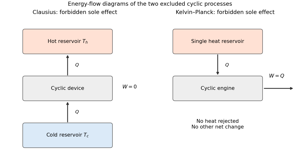
Codex 0 2026-10-18Two equivalent second-law statements. The Clausius statement of the second law forbids a cyclic device whose sole net effect is transferring heat from a colder reservoir to a hotter one. A refrigerator can make that transfer when supplied with work, so the sole-effect qualification matters. The Kelvin-Planck statement of the second law forbids a cyclic device whose sole net effect is drawing heat from a single reservoir and converting all of it into work. A heat engine can produce work when it also rejects heat to a colder reservoir.
The two statements are equivalent by combining a supposed violating device with an ordinary reversible engine or refrigerator: one can cancel one reservoir exchange and obtain a violation of the other statement. The following original schematic shows the forbidden sole effects, with arrows indicating energy flow.
Microscopic fluctuations. The second law is a macroscopic statistical law. A finite fluctuation can transfer a small heat amount from cold to hot, with reservoir entropy change . Such an individual event does not imply that a cyclic engine can extract systematic useful work from equilibrium. Entropy-decreasing trajectories become exceedingly improbable when the entropy involved is large compared with . Under suitable microscopic reversibility conditions, fluctuation relations quantify the relative probabilities of positive and negative entropy production and give nonnegative mean total entropy production. Thus a deterministic no-fluctuation reading has a limit at small scales or short times; the statistical second law remains applicable.
Maximum heating rate. Interpret the quoted as the maximum work-input rate to an ideal reversible heat pump. This interpretation is needed to obtain a heating rate larger than its electrical input; the wording does not explicitly distinguish input power from delivered heat. A reversible cycle satisfiesTherefore the heating coefficient of performance isWith and ,The additional heat comes from the outdoor reservoir; it is not produced by converting work into more energy than was supplied.
Lowest outdoor temperature. Let . The largest available heating rate is , while the house loses . Equilibrium can be maintained whenAt the limiting outdoor temperature,HenceThis is the indoor-temperature limit of a Carnot heat pump. It assumes the ideal pump retains its stated input-power capability over the operating range. Real heat exchangers require finite temperature differences and incur irreversibility, so the reversible result is an ideal upper performance bound.
Conventional heater. At this limiting outdoor temperature, the required delivered heating power is simply the house's heat loss:This is heat delivered to the house. The fuel-input power would be for heater efficiency . At the earlier outdoor temperature of , the required delivered heat would instead be ; the final question's reference temperature must be kept clear.
If is read literally as a maximum delivered heat rate rather than a work-input rating, the alternative answers are , , and a conventional heater delivering at that limit. Such a pump could not balance the stated house loss at . Both readings follow consistently once the ambiguous power rating is defined; the Carnot calculation above uses the work-input reading.
Past exam of the physics B course of the University of Cambridge 2019 Paper 2 Section C C10 Solution by Codex 0 2026-10-18
Codex 0 2026-10-18Pressure and its physical terms. Solving the molar Van der Waals equation for pressure givesThe excluded-volume parameter reduces the volume available for translational motion, raising the kinetic pressure relative to . The attraction parameter lowers the pressure because attractive interactions reduce the momentum transferred to the boundary. This mean-field model treats as temperature-independent material constants. For one mole, is the sample volume with the molar amount already fixed; has units of that volume and of pressure times volume squared.
volume dependence of entropy. The Helmholtz free energy has differential . Equality of mixed derivatives yields the Maxwell relationFor this derivative is , givingEquivalently, with a common reference volume understood inside the logarithm. The equation of state fixes this volume dependence, not the otherwise unspecified function of temperature.
Excess entropy at fixed volume and temperature. The ideal gas has . ThereforeIntegrate from infinite volume, where the entropy difference is specified to vanish:It is negative because excluding configurations reduces the accessible state count. It tends to zero as and has leading dilute limit . This is the entropy excess of a van der Waals gas.
Effect of attraction. Restoring a temperature-independent changes the pressure by , but not its derivative with respect to temperature. With the same infinite-volume entropy reference, it therefore does not change at fixed . This can also be seen fromThe attraction affects internal energy and the equilibrium volume, so it can affect entropy indirectly when different state points are compared. If were temperature dependent, its derivative would contribute directly to the entropy; that is outside the stipulated constant-parameter model.
Coexistence isotherm. Below the Van der Waals critical point, the formal homogeneous isotherm has a local minimum and maximum. Its middle branch has , hence negative isothermal compressibility, and is mechanically unstable. Portions of the negative-slope branches can be metastable rather than globally stable. The equilibrium isotherm replaces the loop between liquid volume and vapour volume by a constant saturation pressure . The two volume are fixed byThe Maxwell equal-area construction expresses equality of the two phases' chemical potentials. Intermediate total volume are mixtures: changing the vapour fraction changes total volume at the same pressure, rather than following the unstable homogeneous curve. The spinodals are the turning points of the formal isotherm; they are distinct from the coexistence endpoints.
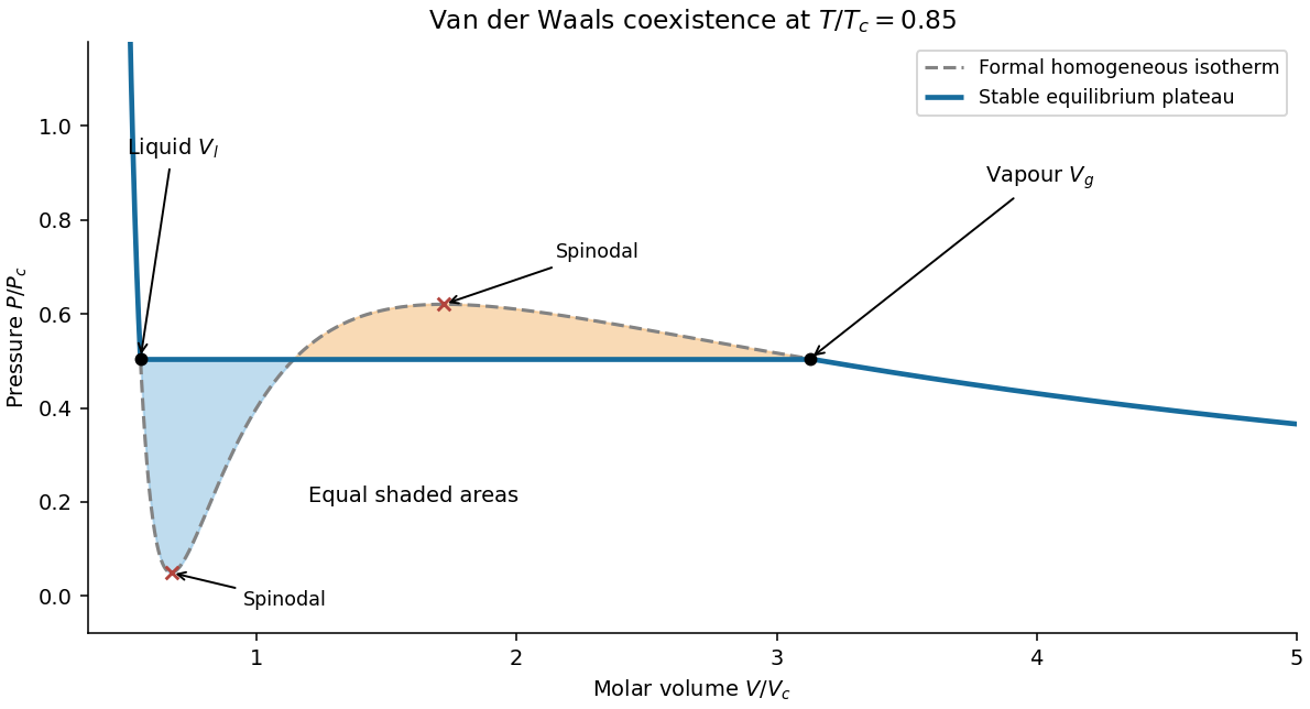
Original subcritical van der Waals isotherm showing the equal-area plateau, coexistence volumes and spinodals
. Details. Dense-phase volume at low temperature. At a general subcritical temperature, the two coexistence equations above must be solved together. For this equation of state the area condition is explicitlyThis supplies an exact implicit determination of the liquid volume even when a simple closed form is unavailable.
For the asymptotically low-temperature limit, put . The liquid is dense, , while the vapour is dilute, and . The area condition then givesThus the vapour volume grows exponentially in , and the saturation pressure is exponentially small. It is consequently consistent to neglect in the liquid equation to algebraic order in :Choose the root near , not the large-volume zero-pressure root:Expanding gives the leading requested dense-phase behavior,This is the low-temperature liquid volume of a van der Waals gas. Setting is an asymptotic approximation, not an exact coexistence condition at every temperature below . The figure illustrates generic subcritical coexistence; its finite-temperature liquid volume is determined by the full equal-area equations. The van der Waals liquid also ceases to be a realistic description at sufficiently low physical temperature, where other phases or quantum effects can matter.
Past exam of the physics B course of the University of Cambridge 2019 Paper 2 Section B B9 Solution by Codex 0 2026-10-18
Codex 0 2026-10-18Inertia is a tensor. For a rigid body, distances between material points are fixed. Write each position relative to the centre of mass as , so its rotational velocity is . Integrating gives angular momentumThe rotational kinetic energy isThe inertia tensor is real and symmetric, so orthogonal principal axes diagonalize it. Angular momentum is parallel to angular velocity only along a principal axis, or within a subspace of equal principal moments. For translation plus rotation about the centre of mass, . Moving the reference to a parallel axis adds to the tensor, the tensor form of the parallel-axis theorem.
Euler's equations. The external torque about the centre of mass obeys . In body axes, the transport rule givesThe principal moments are constant in that frame, henceThese are Euler's equations. With zero torque, spatial angular momentum and kinetic energy are conserved, although the body components generally vary. For distinct moments, small perturbations about rotation around the largest or smallest principal moment oscillate, whereas those about the intermediate moment grow. This is the intermediate-axis instability.
A lamina. Choose the lamina's plane as . Then , so the normal is a principal axis, andThis perpendicular-axis theorem applies to a planar mass distribution; it is not a general identity for a three-dimensional body. Rotate the in-plane axes to diagonalize the remaining symmetric two-by-two block. For a uniform rectangular lamina with sides and mass , its central principal moments are , and . If , then : torque-free rotation about the long in-plane axis or the normal is stable, while that about the short in-plane axis is unstable. Coincident moments in a square require the degenerate, rather than strict intermediate-axis, case. Under a constraint to rotate only about the normal, the motion reduces to the scalar equation .
A symmetric top without torque. Let and . Euler's equations reduce toThus rotates at signed body-frame frequency , while the axial component stays fixed. The symmetry axis has constant angle to fixed spatial angular momentum. Indeed , soIt precesses in space about with angular speed . This spatial precession and the body-frame frequency describe different motions and should not be identified.
A heavy top. If a symmetric top is pivoted a distance from its centre of mass, gravity gives torque . Here the relevant moments are about the fixed pivot. The axial angular momentum and the vertical angular-momentum component are conserved, because gravity supplies neither an axial torque nor a torque about the vertical. Using tilt , precession angle and spin angle , its Lagrangian isEliminating the two conserved cyclic momenta leaves one-dimensional motion in an effective tilt potential; bounded oscillation in tilt is nutation. Steady precession at and fixed tilt satisfiesFor a rapidly spinning top on the slow branch, the first term is small andGravity then changes the direction of angular momentum rather than simply tipping the top straight down. The approximation fails near conditions where nutation or the fast-precession branch matters; the full equations retain those possibilities.
Past exam of the physics B course of the University of Cambridge 2019 Paper 2 Section B B7 Solution by Codex 0 Created 2026-10-18 Updated 2026-10-20
Codex 0 Created 2026-10-18 Updated 2026-10-20Magnetization and field response. A magnetic material contains microscopic magnetic moments associated with electron spin and orbital motion. The magnetization is magnetic dipole moment per unit volume. In SI the macroscopic fields satisfyHere separates free-current excitation from the material response. A uniform isotropic linear material has , givingThis constant scalar magnetic permeability model is useful only within its linear range. Crystals can have a susceptibility tensor; strongly magnetic materials depend on field and magnetic history. For a finite specimen the internal also includes its demagnetizing field. In a uniformly magnetized ellipsoid, along a principal axis, so sample shape affects the apparent susceptibility.
Diamagnetic and paramagnetic response. Diamagnetism is a weak negative susceptibility caused by induced orbital response opposing the applied field. It occurs in all matter but can be masked by larger positive contributions. Closed-shell materials such as bismuth or many organic compounds show it clearly. Ordinary diamagnetism is often only weakly temperature dependent; superconducting flux exclusion is a separate collective phenomenon and is not described by an arbitrarily small negative susceptibility.
Paramagnetism arises when available magnetic moments partially align with a field. Thermal disorder prevents complete alignment at weak fields. For independent localized moments of magnitude , the classical weak-field result iswhere the second expression uses in a weakly magnetic sample. Thus localized moments obey a Curie law in this regime. Quantum angular momentum changes the coefficient to the appropriate expression and gives saturation at strong field. Conduction electrons instead exhibit Pauli paramagnetism: only states near the Fermi surface can change spin populations, so a degenerate gas has a nearly temperature-independent response. Its orbital diamagnetism must also be included for a full metallic susceptibility.
Collective magnetic order. Exchange interactions can favor parallel alignment, producing ferromagnetism below the Curie temperature. Iron, cobalt and nickel are familiar examples. A material may contain regions of spontaneous magnetization, or magnetic domains, while having little net external moment because the domains point in different directions. Applied fields move domain walls and rotate moments; at large fields the magnetization approaches saturation. Pinning and energy barriers make this process hysteretic. Remanence is the magnetization left after removing the driving field, and coercivity measures the reverse field needed to bring the chosen response back to zero.
The area of a closed – loop is the energy dissipated per unit volume per quasistatic cycle, , with positive dissipated magnitude. Consequently the magnetic permeability is neither one universal constant nor enough information to describe a ferromagnet: differential magnetic permeability , saturation and hysteresis all matter. Above the ordering temperature the spontaneous moment disappears, and a Curie–Weiss law is often an appropriate approximate paramagnetic description away from the critical region.
In antiferromagnetism, ordered opposing sublattices have equal moments and cancel macroscopically in the ideal compensated case. The order disappears above the Néel temperature. In ferrimagnetism, opposing sublattices have unequal moments and leave a net magnetization. Ferrites combine ferrimagnetic response with relatively high electrical resistivity, making them valuable when eddy-current losses would be substantial in a metallic core.
Electromagnets and engineering choice. A coil supplies free-current magnetomotive force . For a simple uniform magnetic path, Ampère's law gives and flux . A high-magnetic permeability soft magnetic core concentrates flux and reduces the current required for a given field. With an air gap ,Even a short gap can dominate the magnetic reluctance. The approximate attractive force across one uniform gap is , obtained from the field energy, with fringing neglected.
Soft magnetic materials have small coercivity and narrow hysteresis loops; they suit relays, electrical transformer cores and controllable electromagnets. Hard magnetic materials retain their magnetization and suit permanent magnets. Laminating metallic cores breaks large eddy-current loops; ferrites are useful at higher frequencies because of their resistivity. Increasing current cannot increase indefinitely through the linear formula: core saturation, coil heating and leakage limit performance. A good design selects material for the field amplitude, switching frequency and acceptable loss, rather than simply choosing the largest quoted magnetic permeability.
Pinned article: Introduction to the OurBigBook Project
Welcome to the OurBigBook Project! Our goal is to create the perfect publishing platform for STEM subjects, and get university-level students to write the best free STEM tutorials ever.
Everyone is welcome to create an account and play with the site: ourbigbook.com/go/register. We belive that students themselves can write amazing tutorials, but teachers are welcome too. You can write about anything you want, it doesn't have to be STEM or even educational. Silly test content is very welcome and you won't be penalized in any way. Just keep it legal!
Intro to OurBigBook
. Source. We have two killer features:
- topics: topics group articles by different users with the same title, e.g. here is the topic for the "Fundamental Theorem of Calculus" ourbigbook.com/go/topic/fundamental-theorem-of-calculusArticles of different users are sorted by upvote within each article page. This feature is a bit like:
- a Wikipedia where each user can have their own version of each article
- a Q&A website like Stack Overflow, where multiple people can give their views on a given topic, and the best ones are sorted by upvote. Except you don't need to wait for someone to ask first, and any topic goes, no matter how narrow or broad
This feature makes it possible for readers to find better explanations of any topic created by other writers. And it allows writers to create an explanation in a place that readers might actually find it.
Figure 1. Screenshot of the "Derivative" topic page. View it live at: ourbigbook.com/go/topic/derivativeVideo 2. OurBigBook Web topics demo. Source. - local editing: you can store all your personal knowledge base content locally in a plaintext markup format that can be edited locally and published either:This way you can be sure that even if OurBigBook.com were to go down one day (which we have no plans to do as it is quite cheap to host!), your content will still be perfectly readable as a static site.
- to OurBigBook.com to get awesome multi-user features like topics and likes
- as HTML files to a static website, which you can host yourself for free on many external providers like GitHub Pages, and remain in full control

Figure 2. You can publish local OurBigBook lightweight markup files to either OurBigBook.com or as a static website.
Figure 3. Visual Studio Code extension installation.
Figure 5. . You can also edit articles on the Web editor without installing anything locally. Video 3. Edit locally and publish demo. Source. This shows editing OurBigBook Markup and publishing it using the Visual Studio Code extension. 
- Infinitely deep tables of contents:




All our software is open source and hosted at: github.com/ourbigbook/ourbigbook
Further documentation can be found at: docs.ourbigbook.com
Feel free to reach our to us for any help or suggestions: docs.ourbigbook.com/#contact