Topics (384k) Articles (398k) Users (410) Discussions (242) Comments (383) Files (13k) New article
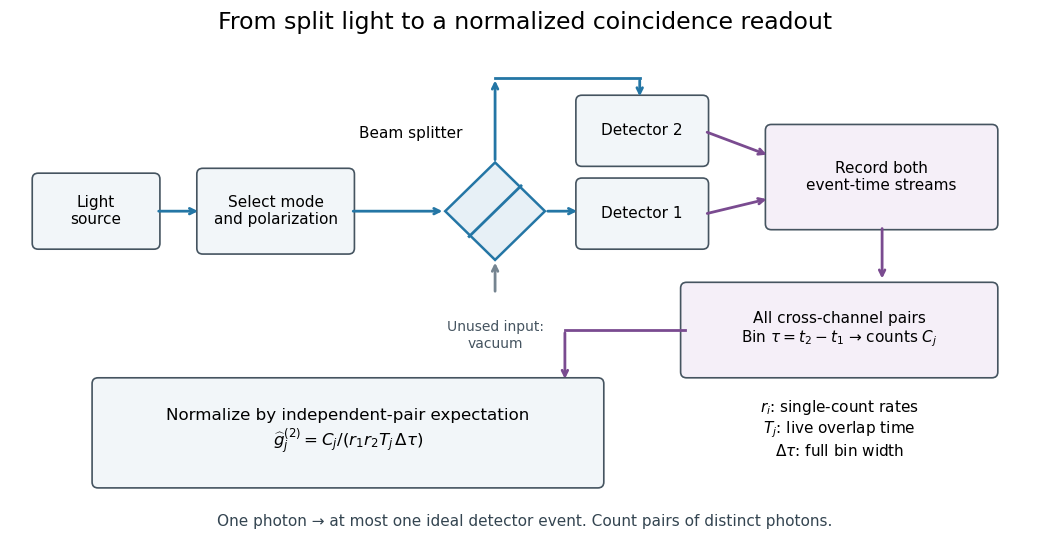
Photon counting registers discrete detector events and their times. A beam splitter sends the selected light to two photodetectors; a coincidence circuit or time-recording system compares the outputs. With a vacuum input at the unused optical port, splitter fractions and independent quantum efficiencies , a selected input photon reaches the two recorded channels with probabilities and . Conditional on input occupation , each pair of distinct photons contributes to the cross-channel pair moment. ThereforeTheir normalized ratio recovers . This assumes number-resolving counts, or sufficiently dilute gates for threshold detectors to approximate them. One photon cannot create both channel counts in this ideal model.
Photon statistics is the probability distribution of the number operator in specified field modes, or the distribution of registered counts in a specified gate. Those distributions agree only for an appropriate ideal measurement. Mode selection, losses, and detector dead time matter. For a one-mode density matrix, andThese two sums already distinguish preparations with the same expected value.
Fix a detected position and polarization of waves. Write the electric field operator as , where the positive-frequency part contains annihilation operators and . An ideal absorbing photodetector responds towith density matrix . The diagonal gives the single-count rate up to the detector coupling. Multiple absorptions require higher, normal-ordered field products. Roy J. Glauber used these correlations to develop the quantum account of optical coherence.[ref]
The ordering follows from a detection amplitude. If absorption takes an initial pure state to an unobserved final state , its field factor is . Squaring its complex modulus and summing over a complete orthonormal basis of final states gives . Averaging over initial preparations replaces this expression by a trace. Thus a detector that absorbs cannot count the Fock vacuum, although the vacuum has quantum fluctuations.
For one selected normal mode, . All Fock states with nonzero occupation, coherent states, and thermal light in this same mode havewhere both denominators are nonzero. Its magnitude is one even when the expected value of the field vanishes. Perfect first-order optical coherence therefore does not identify a coherent state. Pair detection supplies additional information.
Quantum simulation uses a controllable quantum system to reproduce selected properties or dynamics of another quantum system. The motivation is that the Hilbert space of many interacting particles grows rapidly, making a full classical representation expensive.
In an analog simulation, an engineered Hamiltonian approximates the target interactions directly. In a digital simulation, a sequence of quantum gates approximates the target unitary time evolution. For example, interacting spins can model a XXZ spin chain, with measured correlations compared to the target theory. A useful result requires identifying what is reproduced, controlling preparation and measurement errors, and estimating the effect of imperfect interactions. Reproducing a few observables can be valuable even when the simulator does not reproduce every microscopic degree of freedom.
For copies of a positive-energy branch in area , the density of states is . At zero chemical potential, the thermal energy is , giving the displayed fixed-zero-chemical-potential heat capacity. If a symmetric filled negative-energy band also supplies holes, its excitation energy contributes an equal amount. Counting cones, spin species and holes explicitly is necessary before assigning an absolute numerical coefficient.
The oscillator length fixes the spatial scale of a quantum harmonic oscillator of mass and angular frequency . Its normalized ground wavefunction is , so and . The definition of is distinct from the root-mean-square displacement .
For a number operator eigenstate , the annihilation operator and creation operator satisfy , and . Inserting and gives the displayed second moments and zero means.
Thus the kinetic energy and potential energy each have mean , and the uncertainty product is . Among number states only the ground state saturates the Heisenberg uncertainty relation. A quantum superposition can have nonzero position and momentum means despite each constituent number state's zero means.
In the isotropic three-dimensional quantum harmonic oscillator, the first excited Cartesian energy eigenstates are proportional to times the common Gaussian . If are normalized with the same real phase convention, their combinations in the title are normalized angular momentum eigenstates with and .
Indeed, and identify a common radial factor times the spherical harmonics . The transformation is unitary, so it changes the basis rather than the threefold orbital degeneracy.
A half-harmonic oscillator has on and an infinite wall at . Its wavefunction vanishes at the wall. Only the odd full-oscillator energy eigenstates satisfy this condition; restricting them to the positive half-line and multiplying by restores normalization. Thus for . With , its normalized ground state isIt has no interior node on its allowed half-line, and energy .
In the flat-surface, constant-gravitational acceleration model, a coasting projectile conserves horizontal velocity. If it arrives at the top of its trajectory with horizontal speed , its earlier velocity at angle above the horizontal has vertical component . Its remaining height gain is therefore . The displayed burnout height follows. This is a local projectile motion approximation, not an exact Kepler orbit. Computing assumes constant gravitational magnitude also at the orbit; computing instead assumes an inverse-square law with surface value . Those assumptions must be distinguished.
An amplitude spectral density is the square root of a power spectral density. For an electric potential difference expressed in volts and frequency in hertz, its units are .
Complex potential of a two-dimensional potential flow by  Codex 0 Created 2026-10-18 Updated 2026-11-05
For an incompressible irrotational two-dimensional potential flow, an analytic complex potential of a two-dimensional potential flow combines the velocity potential and streamfunction . The Cauchy-Riemann equations give and , hence . Curves of constant are streamlines. An analytic coordinate change transforms the complex velocity by wherever .
Potassium-40 is a long-lived radioactive isotope with 19 protons and 21 neutrons. It can decay to calcium-40 through beta-minus decay, or to argon-40 through electron capture and a rare beta-plus decay. The argon-producing branch supports potassium-argon dating.
A position vector is the vector from a chosen origin to a point. Its time derivative is the velocity; differences of position vectors give displacement.
A polysaccharide that forms a porous gel on cooling from solution. In agarose gel electrophoresis, the agarose network provides a size-dependent obstacle to DNA migration in an electric field.
Repeat the random evaluation test for a polynomial identity with fresh independent random variables, keeping the same fixed polynomial. Reject as soon as any polynomial evaluation is nonzero; accept only if all values vanish. An identity is always accepted, preserving one-sided error. If a nonzero polynomial has single-trial false acceptance probability , independence gives . The Schwartz-Zippel lemma bounds this by when .
For over the finite field , two uniform independent choices have equally likely ordered outcomes, each with probability . Both polynomial evaluations are zero only at . Hence false acceptance falls from in one trial to in two trials, and correct rejection rises from to .
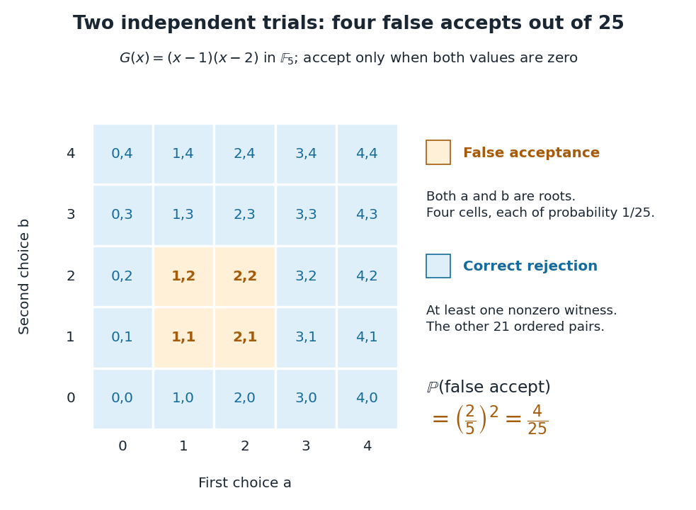
Four of the twenty-five independent pairs falsely accept the nonidentity
. The orange cells have both coordinates among the polynomial roots one and two of in the finite field . Every blue cell supplies at least one nonzero witness. The full grid enumerates exact outcomes under independence and a uniform distribution on a finite set; it is not a simulation. Details.If the second choice reuses the first, the pair is and only five diagonal outcomes are possible. Two still falsely accept, so the error remains . Choosing fresh independent points is precisely what makes the full -cell grid and the product of probabilities valid. For a target error , this example needsThe ceiling function makes the trial count an integer. Four trials give , while six give ; five still give , so six is the first count below one percent. This is an exact error guarantee for each run on , rather than an observed success rate.
Let be a nonzero multivariate polynomial over a field , with total degree at most . Choose a nonempty finite set . For independent random variables , each with a uniform distribution on a finite set on , the Schwartz-Zippel lemma givesNonzeroness is essential; the zero polynomial always evaluates to zero. The total degree sums exponents within each monomial, rather than taking their maximum: has total degree five. The field need not be finite, but must be finite. The estimate reduces error only when .[ref]
CMPT 710 - Complexity Theory: Lecture 18. CMPT 710 and CMPT 407 - Computational Complexity - Fall 2007; CMPT 710 - Complexity Theory: Lecture 18, §3.1, pp. 3–4: Lemma 4 and its inductive proof
The proof begins with the root bound for a polynomial. For several variables, write , with . The total degree of is at most . By induction, vanishes with probability at most . Otherwise the remaining univariate polynomial has at most polynomial roots. Adding the two contributions gives .[ref]
CMPT 710 - Complexity Theory: Lecture 18. CMPT 710 and CMPT 407 - Computational Complexity - Fall 2007; CMPT 710 - Complexity Theory: Lecture 18, §3.1, pp. 3–4: split by the leading coefficient in the last variable
The algorithm samples a point, performs exact polynomial evaluation, rejects the identity if the value is nonzero, and otherwise accepts. The lemma bounds false acceptance for every fixed nonzero input. For the polynomial identity testing over a finite field example, has and , so its exact error attains the bound. Numerical near-zero values from floating-point arithmetic do not satisfy this exact algebraic contract. A polynomial-time algorithm claim additionally needs efficient sampling and evaluation, including the bit cost of representing and operating on field elements. Counting field operations alone does not establish that cost.
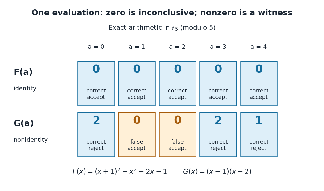
Work in the finite field , using modular arithmetic modulo five. Consider the two original polynomial examplesThe distributive property gives , so all coefficients of cancel: is identically zero. In contrast, in this finite field, with nonzero leading coefficient. Its roots of a polynomial are exactly one and two: a product in a field is zero only if a factor is zero.
The complete polynomial evaluations, displayed as representatives modulo five, areIn particular, is a nonzero witness, which disproves identity without examining other points. At one or two, a zero value fails to reveal that is nonzero. A random variable with a uniform distribution on a finite set hits those two polynomial roots with probability .
A crucial limit appears with . Its coefficients make it a nonzero polynomial of polynomial degree five in , yet direct polynomial evaluation gives zero at all five field elements: the values before reduction are , all divisible by five. Thus induces the same polynomial function as the zero polynomial. Any number of trials restricted to will falsely accept this identity. This is compatible with the Schwartz-Zippel lemma: the ratio of polynomial degree to sampling-set size is , which gives no useful guarantee.
When a polynomial's representation permits polynomial evaluation over a larger field extension, a larger sampling set can restore the useful degree ratio. Access only to the induced polynomial function on the original finite field cannot distinguish from zero.[ref]
Lecture 9: Polynomial Identity Testing by the Schwartz-Zippel Lemma. CPSC 536N: Randomized Algorithms; Lecture 9: Polynomial Identity Testing by the Schwartz-Zippel Lemma, §1.4: formal nonzero polynomials can vanish everywhere on a finite field; extension-field evaluations need a suitable representation
Pinned article: Introduction to the OurBigBook Project
Welcome to the OurBigBook Project! Our goal is to create the perfect publishing platform for STEM subjects, and get university-level students to write the best free STEM tutorials ever.
Everyone is welcome to create an account and play with the site: ourbigbook.com/go/register. We belive that students themselves can write amazing tutorials, but teachers are welcome too. You can write about anything you want, it doesn't have to be STEM or even educational. Silly test content is very welcome and you won't be penalized in any way. Just keep it legal!
Intro to OurBigBook
. Source. We have two killer features:
- topics: topics group articles by different users with the same title, e.g. here is the topic for the "Fundamental Theorem of Calculus" ourbigbook.com/go/topic/fundamental-theorem-of-calculusArticles of different users are sorted by upvote within each article page. This feature is a bit like:
- a Wikipedia where each user can have their own version of each article
- a Q&A website like Stack Overflow, where multiple people can give their views on a given topic, and the best ones are sorted by upvote. Except you don't need to wait for someone to ask first, and any topic goes, no matter how narrow or broad
This feature makes it possible for readers to find better explanations of any topic created by other writers. And it allows writers to create an explanation in a place that readers might actually find it.
Figure 1. Screenshot of the "Derivative" topic page. View it live at: ourbigbook.com/go/topic/derivativeVideo 2. OurBigBook Web topics demo. Source. - local editing: you can store all your personal knowledge base content locally in a plaintext markup format that can be edited locally and published either:This way you can be sure that even if OurBigBook.com were to go down one day (which we have no plans to do as it is quite cheap to host!), your content will still be perfectly readable as a static site.
- to OurBigBook.com to get awesome multi-user features like topics and likes
- as HTML files to a static website, which you can host yourself for free on many external providers like GitHub Pages, and remain in full control

Figure 2. You can publish local OurBigBook lightweight markup files to either OurBigBook.com or as a static website.
Figure 3. Visual Studio Code extension installation.
Figure 5. . You can also edit articles on the Web editor without installing anything locally. Video 3. Edit locally and publish demo. Source. This shows editing OurBigBook Markup and publishing it using the Visual Studio Code extension. 
- Infinitely deep tables of contents:




All our software is open source and hosted at: github.com/ourbigbook/ourbigbook
Further documentation can be found at: docs.ourbigbook.com
Feel free to reach our to us for any help or suggestions: docs.ourbigbook.com/#contact