Consider a single electron of mass $m_e$ and a point atomic nucleus of mass $M$ and positive electric charge $Ze$, with $e>0$ the elementary charge. Use nonrelativistic classical mechanics, omit external fields and interactions with other electrons, and writeHere $\mu$ is the Coulomb two-body reduced mass, ${ϵ}_0$ the vacuum permittivity, and $h$ the Planck constant. The separation $r$ and relative speed $v$ describe the two-particle relative coordinate; neither body is silently pinned in place. The electron's own radius about the centre of mass is $Mr/(M+m_e)$.

For the assumed circular orbit, Coulomb's law provides the required centripetal acceleration, and the imposed orbital angular momentum condition isSubstitute $v=n\hslash /(\mu r)$ into the first equation and cancel $r^{-2}$ to obtainThe kinetic energy is $K=\mu v^2/2=\kappa /(2r)$ and the Coulomb potential energy is $U=-\kappa /r$, with zero energy at infinite separation. HenceThis derives the energy sequence from the stated circular model; the modern Schrödinger equation derivation is the distinct series-termination quantization of the Coulomb radial equation. The radius above scales as $n^2/Z$, whereas the binding energy scales as $\mu Z^2/n^2$. The Bohr radius article supplies the corresponding Coulomb potential length scale. The nonrelativistic assumption requires $v_n\ll c$, with $c$ the speed of light.

For an original numerical example choose $Z=1$, $M=1.67262192369\times 10^{-27}\mathrm{kg}$, $m_e=9.1093837015\times 10^{-31}\mathrm{kg}$, $e=1.602176634\times 10^{-19}\mathrm{C}$, $h=6.62607015\times 10^{-34}\mathrm{J}\mathrm{s}$, ${ϵ}_0=8.8541878128\times 10^{-12}\mathrm{F}{\mathrm{m}}^{-1}$, and $c=299792458\mathrm{m}{\mathrm{s}}^{-1}$. Treat these as stipulated constants for the calculation. They give $\mu /m_e=0.99945568$, $r_1=0.0529465\mathrm{nm}$, $E_1=-13.598287\mathrm{eV}$ and $v_1/c\simeq 0.00730$, where $\mathrm{eV}$ denotes an electronvolt. At $n=2$, $r_2=4r_1$ and $E_2=E_1/4$; the ground-state ionization energy is $-E_1$.

Taking $M\to \infty$ gives $\mu \to m_e$. A finite nuclear mass reduces every binding energy by $\mu /m_e$ and increases each separation by $m_e/\mu$. This follows from relative motion, not a fitted correction to individual spectral lines. Replacing the atomic nucleus by a heavier isotope changes the same factor, providing another check of the model.

The Bloch Hamiltonian acts on the cell-periodic part of a Bloch state at fixed wavevector. If ${\psi }_{n\mathbf{k}}(\mathbf{r})=e^{i\mathbf{k}\cdot \mathbf{r}}{u}_{n\mathbf{k}}(\mathbf{r})$, defineFor a scalar periodic potential, its kinetic term is $(-i\hslash \nabla +\hslash \mathbf{k}{)}^2/(2m)$ on cell-periodic functions.

Solving this family of cell problems produces electronic band structure. In a tight-binding description, the Bloch Hamiltonian is a matrix on the orbitals within a primitive cell, not the full infinite real-space matrix. Basis choices can change its entries without changing the physical band energies. The distinction between the full wavefunction and its periodic factor also matters when computing matrix elements and geometric phases.

Invariance under spatial inversion about a specified origin.

A crystal with $N$ primitive unit cells has $N$ distinct wavevectors in one Brillouin zone. For a rectangular periodic sample, $k_i=2\pi l_i/L_i$, and the product of the numbers of allowed values along the three directions equals the number of cells. Each orbital-derived energy band therefore holds $N$ states per spin orientation, or $2N$ with twofold spin degeneracy. This means two states per primitive cell per spin-degenerate band, independently of how many atoms the cell contains.

William Shockley's proposal used transport through the bulk of a semiconductor, rather than coupling between two surface points. The base must be thin enough for injected minority carriers to reach the collector. Two separately wired diodes do not supply that shared transport region. The proposal was a design principle; producing a working device required further control of material properties.^[ref]

Take a wire segment on the $y$ axis, with source positions ${\mathbf{r}}^{\prime }=(0,s,0)$ for $s_1\le s\le s_2$, and positive electric current along $+y$. Observe at $\mathbf{r}=(a,0,0)$, where $a>0$ is the perpendicular distance to the wire's supporting line. Choose $x$ rightward and $y$ upward, so $+z$ points out of the page. ThenThus the magnetic field points into the page by the right-hand rule. The Biot-Savart law and an elementary antiderivative giveFor an original worked example, choose $s_1=-0.12\mathrm{m}$, $s_2=0.12\mathrm{m}$, $a=0.05\mathrm{m}$, and $I=3\mathrm{A}$. Use ${\mu }_0\approx 4\pi \times 10^{-7}\mathrm{T}m/A$ for these rounded calculations. Each endpoint contributes $0.12/0.13=12/13$, soThese are calculated inputs and output, not laboratory data. The two endpoint angles measured from the perpendicular each have sine $12/13$; this recovers the equivalent endpoint-angle formula without depending on a diagram's angle-sign convention.

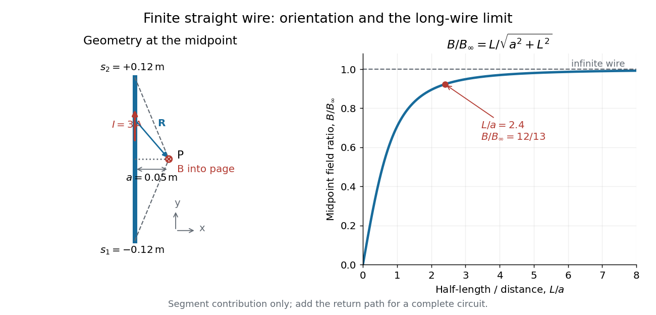
For a segment centered on the perpendicular foot, $s_1=-L$, $s_2=L$. Its magnetic field magnitude isThe limit $L/a\to \infty$ gives $B_{\infty }={\mu }_{0}I/(2\pi a)$, consistent with Ampère's circuital law for an infinite straight wire. In the example, $B_{\infty }=12\mu \mathrm{T}$ and $B/B_{\infty }=12/13$: the infinite-wire value overestimates the segment value by $1/12$, or about $8.33\%$ of the segment value. For $a\gg L$, the isolated segment contribution instead behaves as $B\sim {\mu }_{0}I(2L)/(4\pi a^2)$. The complete localized electrical circuit has a different far-field behavior: return-path contributions cancel this leading segment term, leaving a magnetic dipole field when its magnetic dipole moment is nonzero. Segment and whole-circuit limits must be distinguished.

The SI units check directly: ${\mu }_{0}I/a$ has units $(\mathrm{T}m/A)\mathrm{A}/\mathrm{m}=\mathrm{T}$, the tesla. The apparent divergence as $a\to 0$ is a failure of the thin-wire model near the conductor, not a prediction of infinite magnetic field inside a real wire. This calculation gives only this segment's contribution; include the return wires before comparing with an apparatus.

A current element is the oriented infinitesimal wire contribution $Id{\mathbf{\ell }}^{\prime }$ inside the Biot-Savart law. For uniform axial current density across wire cross-sectional area $A$, $I=JA$ and $d^3{r}^{\prime }=Ad{\ell }^{\prime }$ imply $\mathbf{J}{d}^3{r}^{\prime }=Id{\mathbf{\ell }}^{\prime }$. This reduces a volume integral to a line integral in the thin-wire approximation. It is an integration contribution, not an isolated steady source. Conventional current runs opposite the drift of negatively charged electrons.

For a circular arc of radius $R$ carrying clockwise electric current $I$ and subtending angle $\theta$, with two tangent semi-infinite leads extending on the crossing side of the arc, the axial magnetic field at height $h$ above the centre isThe crossing is insulated. The positive term is from the two leads and the negative term from the arc, with $+z$ out of the clockwise-current plane. The Biot-Savart law yields the lead integral ${\int }_0^{\infty }R(R^2+h^2+s^2{)}^{-3/2}ds=R/(R^2+h^2)$. Cancellation of the axial component gives the title formula, expanding to $\theta =2+h^2/R^2+O(h^4/R^4)$ in radians. This is cancellation of one component away from the plane, not necessarily the entire magnetic field.

A helix-coil transition model assigns local states of a biopolymer to an ordered helical conformation or a disordered coil conformation. Their competing free energies determine the tendency to form a helix, while the cost of boundaries between regions gives cooperativity: forming a new helical run can be less favorable than extending an existing one. A coil state is a class of disordered conformations, not a claim that the whole molecule is an ideal chain. The Zimm-Bragg model is a simple nearest-neighbour statistical model of this competition.

In the reaction displayed here, an electron antineutrino interacts with a proton to produce a Positron and a neutron. It turns an otherwise hard-to-observe incident particle into two products with different detection signatures. A prompt Positron signal followed by neutron capture can identify a candidate much more selectively than a single energy deposit. Inverse beta decay is a weak interaction; the incident electron antineutrino is detected through its reaction products.

A beta particle is an electron or Positron emitted in beta decay. It has the same intrinsic properties as an electron or Positron produced by another process; the name identifies its origin rather than a new particle species.

Unlike a specified two-body alpha transition, ordinary beta emission shares available energy with a neutrino and daughter recoil. The emitted beta particles therefore have a continuous range of kinetic energies. In an applied magnetic field, electrons and positrons curve in opposite senses for the same incident direction. Detector response, energy loss in the sample and collection geometry modify the measured distribution.

Double beta decay changes the atomic number of a nucleus by two while preserving its mass number. The ordinary two-neutrino process can connect even-even nuclear isobars when the intermediate odd-odd nucleus is too heavy for a single beta decay. Neutrinoless variants would violate lepton number and require additional physics.

A nuclide is beta-stable if it has no energetically allowed single beta-minus decay, beta-plus decay, or electron capture to a lower-mass neighboring nuclear isobar, with electron thresholds treated consistently. Beta stability need not imply stability against alpha decay, double beta decay, or nuclear fission.

A nuclear beta decay connects initial and final quantum states through vector and axial-vector parts of the weak charged current. At leading order in the lepton wavelength expansion, Fermi transitions carry lepton-pair spin $S=0$, while Gamow-Teller transitions carry $S=1$. If the lepton pair carries orbital angular momentum $l$, its total angular momentum is $J=l$ for $S=0$, or $J=|l-1|,\dots ,l+1$ for $S=1$. The nuclear states must obey $|J_i-J_f|\le J\le J_i+J_f$, and their parities satisfy ${\pi }_f/{\pi }_i=(-1{)}^l$ in this leading orbital classification. The least permitted $l$ labels the degree of forbiddenness. Real forbidden transitions involve several weak multipole operators; the elementary spin classification does not assert that only one operator or nuclear matrix element exists.

Beryllium-8 has four protons and four neutrons and is unstable against breakup into two alpha particles. Its ground-state resonance lies just above the two-alpha threshold.

This short-lived intermediate is important in the Triple-alpha process: in a sufficiently dense stellar helium environment, a further alpha particle can be captured before breakup. The nuclear resonance therefore connects the structure of a very light unstable nucleus with the production of carbon in stars.

An actual teaching experiment prepares a Kool-Aid stock by weighing powder, transferring it quantitatively into a volumetric flask, and filling to the mark with water. A Genesys 30 spectrophotometer, blanked with water in a cuvette, scans for the peak absorbance wavelength. A Genesys 10 then measures absorbance at that wavelength, with a water reference blank. Each serial dilution transfers $50\mathrm{mL}$ of the preceding chemical solution to a $100\mathrm{mL}$ volumetric flask and fills to the mark; the protocol records the blank and sample readouts and repeats the halving sequence. These are prescribed experimental steps, not a published numerical data set.^[ref]

The experiment tests whether absorbance tracks the prepared concentration. Its concentration is powder mass per final volume, so the calibration does not by itself supply a single dye's molar absorption coefficient. The manual identifies loss of discrimination for very concentrated, very dilute, or very similar samples.^[ref]

To interpret such a calibration, hold cuvette orientation fixed with its clear faces in the light path, keep fingerprints and bubbles out of that path, and keep the geometric length unchanged. Mix each dilution completely. Re-read the reference blank during the sequence and re-read one standard to test drift. A separate preparation of a standard checks errors propagated through serial dilution; repeating only its instrumental reading does not test the transferred volumes. These controls follow from keeping $P_0$, $l$, and $c$ comparable between readings.

Three mechanisms explain why a straight line can fail. First, scattering of light can divert radiant power away from the photodetector, so cloudiness can raise apparent absorbance without the intended absorbing solute. A reference blank removes only losses shared with the sample. Second, stray light reaching the photodetector can make a strongly absorbing sample appear too transmissive. In an original model with extra detected radiant power $s{P}_0$ in both readings,As the ideal transmittance approaches zero, the reported absorbance approaches ${\log }_{10}((1+s)/s)$ for $s>0$. This finite ceiling is a model prediction, not measured instrument performance.

Third, chemical equilibrium can redistribute the absorbing chemical species when dilution, pH, or temperature changes. Even if each chemical species separately follows the Beer-Lambert law, their combined absorbance is $A=l{\sum }_i{\epsilon }_i{c}_i$, where $c_i$ is each species' molar concentration; changing those fractions need not preserve one effective molar absorption coefficient. Thus an unknown should be compared with standards under matching chemical solution conditions, within the tested concentration range. A good linear regression alone does not establish chemical selectivity.

Choose an ideal absorbing chemical species with $\epsilon =8000\mathrm{L}\mathrm{mo}{\mathrm{l}}^{-1}\mathrm{c}{\mathrm{m}}^{-1}$ at a fixed wavelength, and a cuvette with geometric length $l=1\mathrm{cm}$. These are stipulated model parameters. A micromolar molar concentration is $1\mu \mathrm{M}=10^{-6}\mathrm{mol}{\mathrm{L}}^{-1}$, so each additional $25\mu \mathrm{M}$ gives $\Delta A=8000\times 1\times 25\times 10^{-6}=0.2$. Five chosen standards therefore predictThe absorbance graph is a straight line of slope $0.008(\mu \mathrm{M}{)}^{-1}$, while the transmittance graph shows exponential decay. Equal increments of molar concentration multiply transmittance by $10^{-0.2}\approx 0.63096$; they do not subtract a fixed transmitted fraction.

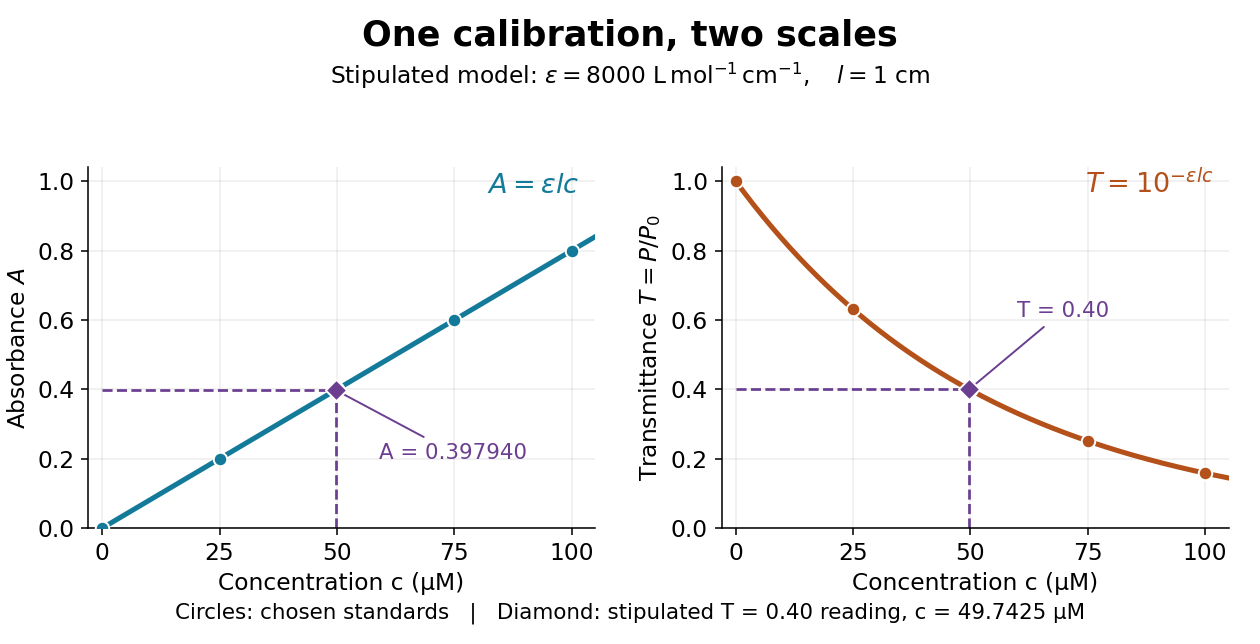
Suppose a measurement returns the stipulated blank-normalized reading $T=0.40$ under those same conditions. The inferred absorbance and molar concentration areThis lies slightly below the $50\mu \mathrm{M}$ standard because $0.40$ is slightly above $10^{-0.4}\approx 0.39811$. A calibration determined experimentally by linear regression may instead have $A=mc+b$. Then use $c=(A-b)/m$, keeping the slope $m$ and intercept $b$ in their measured units. A nonzero intercept calls for checking the reference blank and sample preparation; it does not uniquely identify the cause.

The decadic molar absorption coefficient specifies absorbance per geometric length and molar concentration. With $l$ in centimetres and $c$ in $\mathrm{mol}{\mathrm{L}}^{-1}$, $\epsilon$ has units $\mathrm{L}\mathrm{mo}{\mathrm{l}}^{-1}\mathrm{c}{\mathrm{m}}^{-1}$; its SI unit is ${\mathrm{m}}^2\mathrm{mo}{\mathrm{l}}^{-1}$.^[ref]

The units cancel in $\epsilon lc$. Since $1\mathrm{L}=10^{-3}{\mathrm{m}}^3$ and $1\mathrm{cm}=10^{-2}\mathrm{m}$, one $\mathrm{L}\mathrm{mo}{\mathrm{l}}^{-1}\mathrm{c}{\mathrm{m}}^{-1}$ equals $0.1{\mathrm{m}}^2\mathrm{mo}{\mathrm{l}}^{-1}$. Specify the wavelength and chemical solution conditions when giving a molar absorption coefficient: changing the absorbing chemical species can change it even at fixed total analytical concentration.